CSE 4227 · Prof. Kalpoma · AUST · CLO1 + CLO2 + CLO3

DIP, every dot connected

Every past question of hers (Spring 2022 to Spring 2025, plus the Fall 2025 quizzes) as the real paper image, next to the worked answer and simulator from your lesson pages. Grouped by chapter, each with the pattern she asks in and the formula wall. Fall 2024 and the other examiners' sections are left out.

Night-before revision plan

15 min: the dot map and the cue words. Say out loud which method each story word points to.
2 hours: chapter by chapter. For each one, read the pattern box, then the formula wall. Look at each question image, say the first two lines of the answer, then open Worked answer to check. Don't redo the sums you already know. Run one simulator only if a step feels foggy.
30 min: Q1 theory points and Q3 case bank. Keywords matter more than wording.
10 min: traps and the final checklist. Then sleep.

Click any question image to zoom.

The paper

In plain wordsThree questions. Q1 asks you to explain, Q2 asks you to calculate, Q3 gives a story (a hospital, a satellite, a scanner) and asks which method fits. The same 12 methods answer all three; only the way you write changes.

question	what it wants	choice	how you write it
Q1 theory · 25	define, compare, list effects	any 5 of 6 (one per chapter)	definition → formula → 2–3 points → small sketch
Q2 math · 24	numbers: histogram, filter, compression, chain code / morphology	about 3 of 4	formula → table of every step → final grid / code → one-line comment
Q3 case · 21	a real problem; pick and justify methods	any 3 of 4	problem → method → why → steps (with equation) → result

Time: about 2.5 minutes per mark. A 7-mark case = 17 minutes. Never spend more than 20 minutes on one part.

Where marks hide: the formula line, the working table and the final labelled answer each carry marks on their own. A right answer with no table loses about half.

Dot map: every past question by chapter and CLO

Each row is a chapter. Each column is a section of the paper: Q1 is CLO1 theory, Q2 is CLO2 math, Q3 is CLO3 case. Click a question to jump to its image and answer. Fall 2024 and the other examiners' sections are left out.

chapter	CLO1 · Q1 theory	CLO2 · Q2 math	CLO3 · Q3 case
Pixels, resolution, neighbours and distance decks 01–03	SP25 1b SP24 1a SP22 3a	SP25 1b SP24 1a SP23 2e SP22 3b F21 B4b	–
Point operations deck 04	F23 1b SP23 2d SP22 2a F21 B3b F25 quiz Q1C 1	SP24 3e F23 3d F25 quiz Q1C 2a F25 quiz Q1C 2b	–
Histogram deck 05	F23 1a SP23 2b F22 A2b F25 quiz Q1D 1 F25 quiz Q1D 2a F25 quiz Q2C 1	SP25 2a SP24 2a F23 2a SP23 3b F22 A3b SP22 2b F21 B3a F25 quiz Q1D 2b F25 quiz Q2C 2	–
Spatial filters decks 06–07	SP25 1a SP24 1b F23 2b SP23 2f SP23 3f F22 A1a SP22 1a F21 B4a	SP25 2b SP24 2b F23 2b SP23 2f SP23 3f SP22 1a F21 B4a	F22 A1a
Segmentation decks 08–09	SP25 1e SP24 1e F23 1e SP23 3e F22 A1b SP22 6a F25 quiz Q3D 1	SP25 2d F23 3a SP22 6b	SP25 3a SP24 3a SP23 1b F22 A1b
Chain code (boundary representation) deck 10	SP23 2c F21 B1b	SP25 3d SP24 3d SP23 2c F21 B1b F25 quiz Q3D 2	SP25 3d
Morphology decks 11–12	SP25 1f SP24 1c F22 A2c SP22 4a F21 B1a F25 quiz Q4C 1	SP24 3c F23 2d F23 2e SP23 1a SP23 3c F22 A3c SP22 4b F21 B1a F25 quiz Q4C 2	SP25 3c F23 3b F22 A3c F21 B1a
Compression deck 13	SP25 1d F23 1d SP23 2a F22 A2a SP22 5a	SP25 2c SP25 3b SP24 2c SP24 3b F23 2c F23 3c SP23 3a F22 A3a SP22 1b SP22 5a SP22 5b F21 B2a F21 B2b	–
Colour deck 14	SP25 1c SP24 1d F23 1c SP23 3d SP22 7a SP22 7b	–	–

In plain wordsEvery topic is one stop on the same road: take a picture, make it look better, find the object, describe its shape, store it small. Once you see the road, you know which chapter a question comes from.

1 · Capturedecks 01–03

sampling, quantization, bits, pixels, neighbours, distance

2 · Enhancedecks 04–07

point ops (negative, log, gamma, stretch, slice, bit-plane) → histogram → smooth → sharpen

3 · Find objectsdecks 08–09

edges (gradient, Laplacian, Canny) or regions (threshold, region growing)

4 · Clean shapedecks 11–12

erosion, dilation, opening, closing, boundary, hit-or-miss

5 · Describe shapedeck 10

chain code → CFD → shape number

6 · Store / colourdecks 13–14

Huffman, Golomb, LZW, RLE, RMSE · RGB, CMY, HSI

The same idea shows up twice (connect these dots)

first meeting	second meeting	the link
thresholding s = 1 if r > k (deck 04)	global / iterative threshold (deck 09), binary input for morphology (deck 11)	one cut turns gray into object vs background
contrast stretching (deck 04)	histogram equalization (deck 05)	both spread values over 0…L−1; HE does it automatically from the CDF
mean / Gaussian smoothing (deck 06)	Canny step 1, LoG (deck 08)	smooth first so noise doesn't make fake edges
Laplacian ∇²f (deck 07)	LoG / zero crossings (deck 08)	2nd derivative: thin double edges, sensitive to noise
Sobel / Prewitt gradient (deck 07)	Canny step 2 (deck 08)	1st derivative: edge strength and direction
median filter (deck 06)	salt-and-pepper case questions (Q3)	median ignores extreme 0/255 values and keeps edges
boundary β(A) = A − (A ⊖ B) (deck 11)	chain code walks that boundary (deck 10)	first find the outline, then code it
erosion (deck 11)	hit-or-miss = two erosions (deck 12)	HMT erodes the object with B1 and the background with B2
entropy H (deck 13)	Huffman L_avg (deck 13)	H is the floor: L_avg ≥ H, efficiency = H / L_avg
histogram p(r_k) = n_k/N (deck 05)	probabilities for Huffman and entropy (deck 13)	same counting table, different use
intensity I in HSI (deck 14)	gray-level methods (decks 04–06)	enhance I only, keep H and S, colours stay true

Cue words: story word, then method

In plain wordsCase questions hide the method inside a story. Spot the problem word, map it to the method, then justify with one line of how the method works. Learn this table and Q3 becomes matching.

Enhancement stories

you read	it means	you write / use
too dark, underexposed X-ray / MRI, details hidden in shadows	dark values squashed together	log or gamma γ < 1; or histogram equalization
washed out, too bright, aerial photo, faded	bright values squashed together	gamma γ > 1 (3.0–4.0 on the slides)
low contrast, dull, narrow histogram	values use only part of 0…L−1	contrast stretching or histogram equalization
highlight a range: tumor, bone [120, 200], water in satellite	one band of gray levels matters	gray-level slicing: give both approaches (background 0, or keep r)
huge dynamic range, Fourier spectrum	values 0 to 10⁶ won't fit 0–255	log transform
negative film, white lesions in dark mammogram	dark ↔ light swap helps viewing	negative s = L−1−r
hidden watermark, which bits matter, compress by bits	image = stack of bit planes	bit-plane slicing: top planes carry the shape
want the look of another image	target histogram given	histogram matching (specification)

Noise and sharpness stories

you read	it means	you write / use
salt-and-pepper, impulse noise, black and white dots	isolated extreme 0 / 255 pixels	median filter 3×3 (keeps edges)
Gaussian noise, grainy, random noise	every pixel slightly off	mean / weighted average / Gaussian filter (blurs a bit)
only pepper (black dots) / only salt (white dots)	one-sided impulses	max filter removes pepper, min filter removes salt
blurred, fine detail, sharpen, faded ink edges	edges too soft	Laplacian g = f − ∇²f, or unsharp masking / high-boost
find edges / outline of an organ, crack, road edge	big change in intensity	Sobel / Prewitt gradient, best: Canny
noisy image but need thin, clean, connected edges	edge detector that resists noise	Canny (smooth, gradient, NMS, double threshold, hysteresis)
straight lines: roads, lanes, fracture lines	pixels lying on a line	line masks (−1 −1 −1 / 2 2 2) or Hough transform (one line: votes in (ρ, θ))

Segmentation stories

you read	it means	you write / use
separate object from background, text from paper	two intensity groups	thresholding; iterative T = ½(μ₁ + μ₂)
uneven illumination, shadow on the document	one T can't fit everywhere	local / adaptive threshold (T from each neighbourhood)
group similar pixels from a seed point, tumor region	grow from a known pixel	region growing: \|neighbour − pixel it grows from\| ≤ T
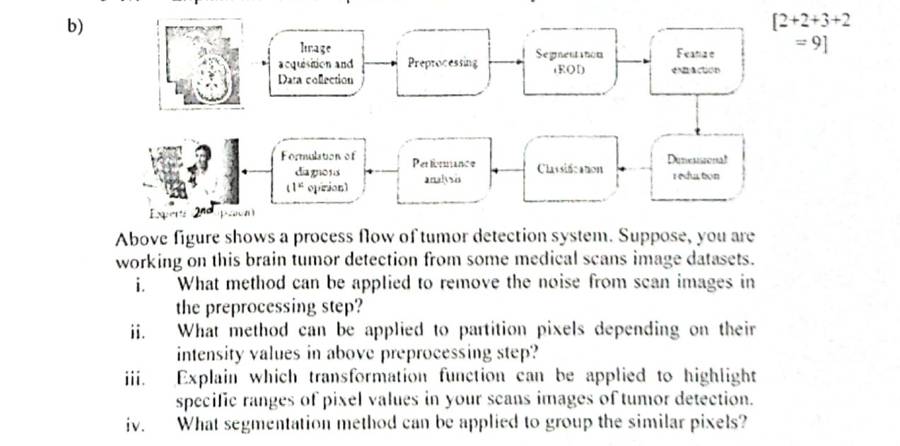
"partition pixels depending on intensity"	the words for thresholding	thresholding (SP23 Q1(b)ii)
"groups similar pixels"	the words for region-based	region growing or split & merge (SP23 Q1(b)iv)

Shape stories (binary images)

you read	it means	you write / use
broken characters, gaps in roads, cracks to join	small breaks in the object	dilation (or closing to keep thickness)
small bright spots, specks, small particles to remove	objects smaller than the SE	opening (erode, then dilate)
small holes inside objects, reflections to fill	background specks inside the object	closing (dilate, then erode)
touching coins, count objects	thin necks join the objects	erosion to split, then count connected components
outline / boundary of roads, organ edge (binary)	the object's border pixels	boundary β(A) = A − (A ⊖ B)
find corners, end points, a fixed pattern	match object AND background	hit-or-miss A ⊛ B = (A ⊖ B₁) ∩ (Aᶜ ⊖ B₂)
recognise a shape whatever its rotation / start	describe the boundary by numbers	chain code → CFD → NCFD (shape number)

Storage and colour stories

you read	it means	you write / use
medical, legal, must not lose any detail	lossless only	Huffman, LZW, RLE, Golomb, arithmetic
many repeating patterns / colours, bitmap, fixed-length codes	the same sequences come back	LZW (dictionary, 9-bit codes)
long runs of the same value, fax, binary documents	consecutive equal pixels	RLE (value, run length)
some gray levels far more common than others	unequal probabilities	Huffman (short codes for frequent values)
small integers / prediction errors, geometric spread	small values common	Golomb G_m(n)
whole message as one number	non-block code	arithmetic coding
how good is the decompressed image?	fidelity criterion	RMSE (objective) or rating scale (subjective)
printing, ink, printer	subtractive colour	CMY / CMYK
monitor, camera, display	additive colour	RGB
segment by colour, lighting changes, describe colour like humans	separate colour from brightness	HSI (use Hue)

TrapWhen a case lists four methods (SP25 Q3(d): chain code, histogram, Hough, power-law), give each one line of what it does, one line of how it helps here, and one limitation. That is the 3-part pattern she marks.

1. Pixels, resolution, neighbours and distance

decks 01–03 · 6 past questions

The pattern: how she asks it

Q1 (4 marks): 4- vs 8- vs m-connectivity, then count the connected components of a small 0/1 grid (SP25 1b). Sampling vs quantization and image types also come here.
Q2 small part: D4 / D8 / De between two pixels, or the shortest 4-, 8- or m-path through a set V (SP23 2e, SP22 3b, SP24 1a).
Arithmetic: bits = M × N × k, levels L = 2^k; zoom by pixel replication / nearest neighbour.

Connects to: m-adjacency comes back in chain code (the boundary is a path) and in morphology (connected components, coin counting).

type	CLO	times	where
Distances D4/D8/De, paths, adjacency, components	CLO2	5	SP25 1b, SP24 1a, SP23 2e, SP22 3b, F21 B4b
Neighbours, adjacency, m-connectivity, distance properties	CLO1	2	SP25 1b, SP24 1a
Fundamentals: sampling, quantization, intensity levels, image types	CLO1	1	SP22 3a

Formula wall: every formula with a worked line

what	formula	one worked line
gray levels	L = 2^k, range 0 … L−1	k = 12 → L = 4096, range 0–4095
image size	b = M × N × k bits (÷ 8 = bytes)	1024 × 768 × 12 = 9,437,184 bits = 1,179,648 bytes
nearest-neighbour zoom	position = ⌈i × old / new⌉, i = 1…new	3×3 → 5×5: ⌈0.6 i⌉ = 1 2 2 3 3 (copy those rows / columns)
city-block D₄	\|x − s\| + \|y − t\|	p(1,2), q(4,6): 3 + 4 = 7
chessboard D₈	max(\|x − s\|, \|y − t\|)	max(3, 4) = 4
Euclidean D_e	√[(x − s)² + (y − t)²]	√(9 + 16) = 5

Sampling = digitise coordinates (spatial resolution, blocky if too few). Quantization = digitise amplitude (gray-level resolution, false contouring if too few).
4-adjacent: q in N₄(p). 8-adjacent: q in N₈(p). m-adjacent: q in N₄(p), or q in N_D(p) and N₄(p) ∩ N₄(q) has no pixel in V. m removes the double paths of 8-adjacency.
Distance properties: D ≥ 0 (= 0 only if p = q), D(p,q) = D(q,p), D(p,z) ≤ D(p,q) + D(q,z). Always D₄ ≥ D_e ≥ D₈.

Past questions: look, recall, then open the answer

SP25 1bCLO1 · Neighbours, adjacency, m-connectivity, distance properties · 2CLO2 · Distances D4/D8/De, paths, adjacency, components · 2

State the difference between 4-neighbor, 8-neighbor and m-connectivity. Given a 4x4 binary image segment [(1010),(0101),(1010),(0101)], determine the number of connected components under each connectivity type and discuss the effect of diagonal adjacency on these components.

Worked answer (deck 03)

SP25 Final Q1(b)4 marks

State the difference between 4-neighbour, 8-neighbour and m-connectivity. For the 4×4 binary image [1010; 0101; 1010; 0101], find the number of connected components under each connectivity and discuss the effect of diagonal adjacency.

4-connectivity: only the up/down/left/right neighbours link pixels. 8-connectivity: the four diagonal neighbours link too. m-connectivity: 4-neighbours always link; a diagonal neighbour links only if the two pixels have no common 4-neighbour with a value in V (removes the double paths of 8-connectivity).

1	0	1	0
0	1	0	1
1	0	1	0
0	1	0	1

V = {1}

Every 1 has only 0s as 4-neighbours, so with 4-connectivity each 1 is alone: 8 components. Every 1 touches other 1s diagonally, so 8-connectivity joins all of them: 1 component. For each diagonal pair the two shared 4-neighbours are 0 (not in V), so every diagonal link is m-adjacent as well: 1 component.

Effect of diagonal adjacency: it merges pixels that touch only at corners, dropping the count from 8 to 1. m-connectivity keeps those joins here and only removes redundant (ambiguous) diagonal links where a 4-connection already exists.

SP24 1aCLO1 · Neighbours, adjacency, m-connectivity, distance properties · 2CLO2 · Distances D4/D8/De, paths, adjacency, components · 3

What are the properties of the Distance Function for Distance Metrics if there are 3 pixels a, b and c? How to calculate the distances City Block, Chess Board, Euclidean between two pixels a and b? [2+3]

Worked answer (deck 03)

SP24 Final Q1(a)2 + 3 marks

What are the properties of the distance function for 3 pixels a, b and c? How are the city-block, chessboard and Euclidean distances between a and b calculated?

Properties: D(a,b) ≥ 0 with D(a,b) = 0 iff a = b; D(a,b) = D(b,a); D(a,c) ≤ D(a,b) + D(b,c).

For a = (x, y), b = (s, t): city block D₄ = |x − s| + |y − t|; chessboard D₈ = max(|x − s|, |y − t|); Euclidean D_e = √[(x − s)² + (y − t)²]. Example a = (0,0), b = (3,4):

D₄(a,b) = |0 − 3| + |0 − 4| = 7 (city block)
D₈(a,b) = max(|0 − 3|, |0 − 4|) = max(3, 4) = 4 (chessboard)
D_e(a,b) = √[(0 − 3)² + (0 − 4)²] = √25 = 5.0000 (Euclidean)

SP23 2eCLO2 · Distances D4/D8/De, paths, adjacency, components · 5

5x4 image [9,34,20,0,16,21,50,5,5,6,11,15,7,8,10,2,8,7,9,0], V={10,20,9,7,0,5,1,3}. i) Does any 8-path exist between 9th and 19th pixels? Explain. ii) Find their City Block, Chess Board, Euclidean distances. [2+3]

Worked answer (deck 03)

SP23 Final Q2(e)2 + 3 marks

5×4 image [9, 34, 20, 0, 16, 21, 50, 5, 5, 6, 11, 15, 7, 8, 10, 2, 8, 7, 9, 0], V = {10, 20, 9, 7, 0, 5, 1, 3}. (i) Does an 8-path exist between the 9th and the 19th pixels? (ii) Their city-block, chessboard and Euclidean distances.

5×4 = 5 rows × 4 columns. Counting row by row from 1: the 9th pixel is (2,0) = 5 and the 19th is (4,2) = 9.

9	34	20	0
16	21	50	5
5	6	11	15
7	8	10	2
8	7	9	0

grey = not in V

(i) Yes: (2,0)=5 → (3,0)=7 → (4,1)=7 → (4,2)=9. All values are in V and each step goes to an 8-neighbour (the step (3,0) → (4,1) is diagonal).

(ii)

D₄(p,q) = |2 − 4| + |0 − 2| = 4 (city block)
D₈(p,q) = max(|2 − 4|, |0 − 2|) = max(2, 2) = 2 (chessboard)
D_e(p,q) = √[(2 − 4)² + (0 − 2)²] = √8 = 2.8284 (Euclidean)

Try it, step by step: SP23 Q2(e): the 8-path from the 9th to the 19th pixel.

SP22 3aCLO1 · Fundamentals: sampling, quantization, intensity levels, image types · 5

i) Mention two techniques that made the digital representation of analog world possible [3]. ii) 'The more intensity levels used, the finer level of detail discernible in an image' - explain why [2].

Worked answer (deck 01–02)

SP22 Final Q3(a)3 + 2 marks

(i) Mention two techniques that made the digital representation of the analog world possible. (ii) “The more intensity levels used, the finer the level of detail discernible in an image.” Explain why.

(i) Sampling: measuring the continuous scene only at a grid of points, which digitizes the coordinates and fixes the spatial resolution M × N. Quantization: rounding each sampled brightness to one of L discrete levels (L = 2^k), which digitizes the amplitude. Together they turn the analog picture into a matrix of integers.

(ii) With more levels the step between neighbouring gray values is smaller, so small brightness differences (soft shading, fine texture) get different numbers and stay visible. With few levels, many different intensities are rounded to the same value; smooth areas turn into flat bands with visible jumps between them (false contouring, slides 30–34), and fine detail is lost.

SP22 3bCLO2 · Distances D4/D8/De, paths, adjacency, components · 8

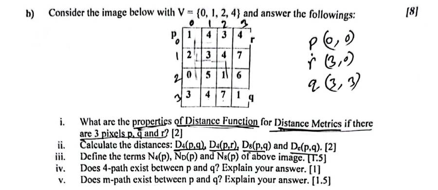
4x4 image [[1,4,3,4],[2,3,4,7],[0,5,1,6],[3,4,7,1]], V={0,1,2,4}; p=(0,0) top-left, r=(0,3) top-right, q=(3,3) bottom-right. i) Properties of distance function for p,q,r [2] ii) D4(p,q), D4(p,r), D8(p,q), De(p,q) [2] iii) N4(p), ND(p), N8(p) [1.5] iv) 4-path between p and q? [1] v) m-path between p and q? [1.5]

Worked answer (deck 03)

SP22 Final Q3(b)2 + 2 + 1.5 + 1 + 1.5 marks

4×4 image, V = {0, 1, 2, 4}; p = (0,0) top-left, r = (0,3) top-right, q = (3,3) bottom-right. (i) Properties of the distance function for p, q, r. (ii) D₄(p,q), D₄(p,r), D₈(p,q), D_e(p,q). (iii) N₄(p), N_D(p), N₈(p). (iv) Is there a 4-path between p and q? (v) An m-path between p and q?

1	4	3	4
2	3	4	7
0	5	1	6
3	4	7	1

image; grey cells are not in V

(i) D(p,q) ≥ 0 and = 0 only if p = q; D(p,q) = D(q,p); D(p,r) ≤ D(p,q) + D(q,r).

(ii) D₄(p,q) = |0 − 3| + |0 − 3| = 6; D₄(p,r) = |0 − 0| + |0 − 3| = 3; D₈(p,q) = max(3, 3) = 3; D_e(p,q) = √(9 + 9) = 4.2426.

(iii) p is a corner, so the other neighbours fall outside: N₄(p) = {(1,0) = 2, (0,1) = 4}; N_D(p) = {(1,1) = 3}; N₈(p) = {(1,0) = 2, (0,1) = 4, (1,1) = 3}.

(iv) 4-path: none. From p, the 4-neighbours in V are (0,1) = 4 and (1,0) = 2; from them every 4-step leads to 3, 5 or 7 (not in V), so q cannot be reached.

(v) m-path: (0,0)=1 → (0,1)=4 → (1,2)=4 → (2,2)=1 → (3,3)=1. Check the diagonal (0,1) → (1,2): shared 4-neighbours (0,2) = 3 and (1,1) = 3 are not in V, so the step is m-adjacent; likewise (2,2) → (3,3) with (2,3) = 6, (3,2) = 7.

Try it, step by step: SP22 Q3(b): the 4-path fails; the m-path goes round through the diagonals.

F21 B4bCLO2 · Distances D4/D8/De, paths, adjacency, components · 6

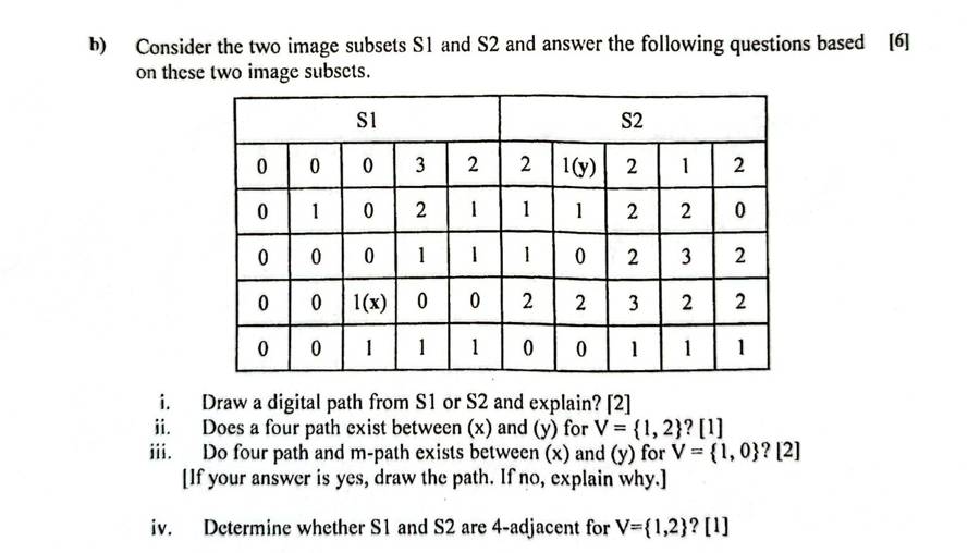
Subsets S1 [[0,0,0,3,2],[0,1,0,2,1],[0,0,0,1,1],[0,0,1(x),0,0],[0,0,1,1,1]] and S2 [[2,1(y),2,1,2],[1,1,2,2,0],[1,0,2,3,2],[2,2,3,2,2],[0,0,1,1,1]] side by side. i) Draw a digital path, explain [2] ii) 4-path between x and y for V={1,2}? [1] iii) 4-path and m-path for V={1,0}? [2] iv) Are S1 and S2 4-adjacent for V={1,2}? [1]

Worked answer (deck 03)

F21 Final B4(b)2 + 1 + 2 + 1 marks

S1 (columns 0–4) and S2 (columns 5–9) side by side; x = (3,2) in S1, y = (0,6) in S2. (i) Define a digital path. (ii) Is there a 4-path between x and y for V = {1, 2}? (iii) 4-path and m-path for V = {0, 1}. (iv) Are S1 and S2 4-adjacent for V = {1, 2}?

0	0	3	2	2	1	2	1	2
1	0	2	1	1	1	2	2	0
0	0	1	1	1	0	2	3	2
0	1	0	0	2	2	3	2	2
0	1	1	1	0	0	1	1	1

x = (3,2), y = (0,6)

(i) A sequence of distinct pixels from x to y, each adjacent (4, 8 or m) to the next, all with values in V; the number of steps is its length.

(ii) V = {1, 2}: no 4-path. x's 4-neighbours are 0, 0, 1 and 0; the 1 below leads only to more 1s at the bottom that never reach the top-right through 1s and 2s.

(iii) V = {0, 1}: 4-path (3,2)=1 → (2,2)=0 → (2,3)=1 → (2,4)=1 → (1,4)=1 → (1,5)=1 → (1,6)=1 → (0,6)=1; m-path (3,2)=1 → (2,2)=0 → (2,3)=1 → (2,4)=1 → (1,4)=1 → (1,5)=1 → (1,6)=1 → (0,6)=1 (the same here: a 4-path is also an m-path).

(iv) Yes: column 4 of S1 and column 5 of S2 touch with values in {1, 2}: row 0: 2 | 2, row 1: 1 | 1, row 2: 1 | 1.

Try it, step by step: F21 B4(b): change nothing for V = {0, 1}: watch the 4-path being found.

More worked examples: slides and other examiners (10)

Slide 25 · answer the questions (deck 01–02)

Slide 25 · answer the questionsworked

Q1 1 bit → 2¹ = 2 levels (0, 1). Q2 2 bits → 4 levels. Q3 p bits → 2^p levels. Q4 256 intensities → log₂ 256 = 8 bits.

Q5 3-bit 5×5 image: gray-level resolution L = 2³ = 8 levels (range 0–7); spatial resolution 5 × 5 = 25 pixels; size b = 5 × 5 × 3 = 75 bits; bit depth 3.

F22 Final B4(b) · F21 Final A3(b) (other examiners' papers) (deck 01–02)

F22 Final B4(b) · F21 Final A3(b) (other examiners' papers)5 · 6 marks

F22: define sampling and quantization; bits for 512 intensities; spatial resolution and bit size of a 7×5 image. F21: a 256×256 image with 64 gray levels: bit depth and size in bytes; Mach band effect; index image; why more levels show finer detail.

F22: sampling digitizes coordinates, quantization digitizes amplitude. 512 intensities → k = log₂ 512 = 9 bits. A 7×5 image has spatial resolution 7 × 5 = 35 pixels; with 9 bits per pixel, b = 7 × 5 × 9 = 315 bits.

F21: 64 levels → k = log₂ 64 = 6 bits; b = 256 × 256 × 6 = 393,216 bits = 393,216 / 8 = 49,152 bytes (48 KB). Mach band effect: at the boundary between two flat bands of different brightness the eye sees a darker strip on the dark side and a brighter strip on the light side (overshoot/undershoot) that is not in the image. Index image: each pixel stores an index into a colour table (palette) holding the actual RGB values. The last part is the same as SP22 (ii) above.

Slides 49–54 · 3×3 → 6×6 (deck 01–02)

Slides 49–54 · 3×3 → 6×6worked

Step 1 · ratios: Ratio_row = 3/6, Ratio_col = 3/6.

Step 2 · positions = ratio × [1 … 6], rounded up (ceil):

rows: 3/6 × [1 2 3 4 5 6] = [0.5 1 1.5 2 2.5 3] → ceil → [1 1 2 2 3 3]
cols: 3/6 × [1 2 3 4 5 6] = [0.5 1 1.5 2 2.5 3] → ceil → [1 1 2 2 3 3]

Step 3 · copy: output pixel (i, j) = old pixel (row position i, column position j).

10	4	22
2	18	7
9	14	25

original 3×3

10	10	4	4	22	22
10	10	4	4	22	22
2	2	18	18	7	7
2	2	18	18	7	7
9	9	14	14	25	25
9	9	14	14	25	25

output 6×6

Try it, step by step: the slide example. Change the new size (e.g. 5×5, 7×7, 9×9) to see how the positions change; the class-work matrices are solved just below.

Slide 55 · class work (deck 01–02)

Slide 55 · class worksolved

2×2 → 5×5

Step 1 · ratios: Ratio_row = 2/5, Ratio_col = 2/5.

Step 2 · positions = ratio × [1 … 5], rounded up (ceil):

rows: 2/5 × [1 2 3 4 5] = [0.4 0.8 1.2 1.6 2] → ceil → [1 1 2 2 2]
cols: 2/5 × [1 2 3 4 5] = [0.4 0.8 1.2 1.6 2] → ceil → [1 1 2 2 2]

Step 3 · copy: output pixel (i, j) = old pixel (row position i, column position j).

1	4
3	7

original 2×2

1	1	4	4	4
1	1	4	4	4
3	3	7	7	7
3	3	7	7	7
3	3	7	7	7

output 5×5

3×3 → 9×9

Step 1 · ratios: Ratio_row = 3/9, Ratio_col = 3/9.

Step 2 · positions = ratio × [1 … 9], rounded up (ceil):

rows: 3/9 × [1 2 3 4 5 6 7 8 9] = [0.333 0.667 1 1.33 1.67 2 2.33 2.67 3] → ceil → [1 1 1 2 2 2 3 3 3]
cols: 3/9 × [1 2 3 4 5 6 7 8 9] = [0.333 0.667 1 1.33 1.67 2 2.33 2.67 3] → ceil → [1 1 1 2 2 2 3 3 3]

Step 3 · copy: output pixel (i, j) = old pixel (row position i, column position j).

1	4	3
7	2	3
5	6	0

original 3×3

1	1	1	4	4	4	3	3	3
1	1	1	4	4	4	3	3	3
1	1	1	4	4	4	3	3	3
7	7	7	2	2	2	3	3	3
7	7	7	2	2	2	3	3	3
7	7	7	2	2	2	3	3	3
5	5	5	6	6	6	0	0	0
5	5	5	6	6	6	0	0	0
5	5	5	6	6	6	0	0	0

output 9×9

4×4 → 7×7

Step 1 · ratios: Ratio_row = 4/7, Ratio_col = 4/7.

Step 2 · positions = ratio × [1 … 7], rounded up (ceil):

rows: 4/7 × [1 2 3 4 5 6 7] = [0.571 1.14 1.71 2.29 2.86 3.43 4] → ceil → [1 2 2 3 3 4 4]
cols: 4/7 × [1 2 3 4 5 6 7] = [0.571 1.14 1.71 2.29 2.86 3.43 4] → ceil → [1 2 2 3 3 4 4]

Step 3 · copy: output pixel (i, j) = old pixel (row position i, column position j).

1	4	3	7
2	3	4	5
2	6	4	3
4	7	1	0

original 4×4

1	4	4	3	3	7	7
2	3	3	4	4	5	5
2	3	3	4	4	5	5
2	6	6	4	4	3	3
2	6	6	4	4	3	3
4	7	7	1	1	0	0
4	7	7	1	1	0	0

output 7×7

Slide 11 · practice (deck 03)

Slide 11 · practiceworked

For the 7×7 image (rows and columns numbered from 1, as on the slide) find N₄(3,4), N_D(3,4), N₈(3,4), N₄(1,1), N₄(4,1), N₈(7,7).

49	47	48	45	46	43	42
47	41	43	44	45	49	48
48	47	49	45	50	43	49
49	49	49	49	49	50	50
48	48	48	48	48	49	50
48	48	49	50	50	50	49
49	50	50	51	51	50	50

rows/columns 1–7; (3,4) = 45 outlined

N₄(3,4) = {(2,4) = 44, (4,4) = 49, (3,3) = 49, (3,5) = 50}
N_D(3,4) = {(2,3) = 43, (2,5) = 45, (4,3) = 49, (4,5) = 49}
N₈(3,4) = {(2,4) = 44, (4,4) = 49, (3,3) = 49, (3,5) = 50, (2,3) = 43, (2,5) = 45, (4,3) = 49, (4,5) = 49}
N₄(1,1) = {(2,1) = 47, (1,2) = 47}: a corner, only 2 neighbours inside
N₄(4,1) = {(3,1) = 48, (5,1) = 48, (4,2) = 49}: on the left border, 3 inside
N₈(7,7) = {(6,7) = 49, (7,6) = 50, (6,6) = 50}: a corner, 3 inside

Slide 21 · 4- and 8-adjacency (deck 03)

Slide 21 · 4- and 8-adjacencyworked

V = {0, 1, 2, 3, 5}. A = (0,0), B = (0,1), E = (1,1), C = (2,2), D = (3,3). Which pairs are 4-adjacent / 8-adjacent?

4	2	3	2
3	3	1	3
2	3	5	2
2	1	2	5

A=4 at (0,0), B=2, E=3, C=5, D=5

pair	neighbours?	values in V?	4-adjacent	8-adjacent
A, B	yes (4-neighbours)	A = 4 ∉ V	no	no
A, C	no	A = 4 ∉ V	no	no
B, C	no: (0,1) and (2,2) are 2 rows apart	yes	no	no
C, D	diagonal	yes	no	yes
C, E	diagonal	yes	no	yes

Slide 22 · m-adjacency (deck 03)

Slide 22 · m-adjacencyworked

V = {0, 1, 2, 3, 5}. A = (0,0) = 4, B = (0,1) = 2, C = (2,2) = 5, D = (3,3) = 0. Which pairs are m-adjacent?

4	2	3	2
3	3	1	3
2	3	5	4
2	1	6	0

C = 5 at (2,2), D = 0 at (3,3)

A, B / A, C: no, A = 4 ∉ V. B, C: not neighbours. C, D: D ∈ N_D(C); N₄(C) ∩ N₄(D) = {(2,3) = 4, (3,2) = 6}, and neither 4 nor 6 is in V, so C and D are m-adjacent.

Slide 20 · 4-, 8- and m-paths (deck 03)

Slide 20 · 4-, 8- and m-pathsworked

V = {1, 2}; p = (1,3), q = (3,3) in the slide's numbering (top-right and bottom-right).

0	1	1
0	2	0
0	0	1

rows/cols 1–3 on the slide; here (0,2) = p and (2,2) = q

8-path: two exist: (1,3) → (1,2) → (2,2) → (3,3) and (1,3) → (2,2) → (3,3). That ambiguity is what m-adjacency removes.

m-path: only (1,3) → (1,2) → (2,2) → (3,3). The diagonal step (1,3) → (2,2) is not allowed because they share the 4-neighbour (1,2) = 1 ∈ V. The step (2,2) → (3,3) is allowed: their shared 4-neighbours (2,3) and (3,2) are both 0.

4-path: absent: from (2,2) the only way down is through 0s.

Try it, step by step: slide 20: switch between 4-, 8- and m-paths and watch which steps are allowed.

Slide 23 · m-connected path (deck 03)

Slide 23 · m-connected pathworked

V = {1, 2}. Find the m-connected path between p (bottom-left) and q (top-right). Is a 4-connected path possible?

4	2	3	2
3	3	1	3
2	3	2	2
2	1	2	3

p = (3,0), q = (0,3)

4-path: none. m-path: (3,0)=2 → (3,1)=1 → (3,2)=2 → (2,2)=2 → (1,2)=1 → (0,3)=2, i.e. 2(p) → 1 → 2 → 2 → 1 → 2(q) as on the slide.

Try it, step by step: slide 23: the m-path, step by step. Try 4-path too: it fails.

Slide 32 · practice (deck 03)

Slide 32 · practiceworked

p = (3,4), q = (6,7). Find D₄, D₈, D_e.

D₄(p,q) = |3 − 6| + |4 − 7| = 6 (city block)
D₈(p,q) = max(|3 − 6|, |4 − 7|) = max(3, 3) = 3 (chessboard)
D_e(p,q) = √[(3 − 6)² + (4 − 7)²] = √18 = 4.2426 (Euclidean)

2. Point operations: negative, log, gamma, stretching, slicing, bit planes

deck 04 · 9 past questions

The pattern: how she asks it

Q1: short notes on negative / log / power-law; the piecewise (r1,s1), (r2,s2) cases: identity, threshold, stretch (SP23 2d, SP22 2a, F21 B3b).
Q2: bit-plane slicing of a small grid (SP25 2b i, SP24 2b i); gray-level slicing map (F25 quiz).
Q3 case: dark or washed-out X-ray, so power-law with γ < 1 or > 1, plus contrast stretching numbers (F23 3d, SP24 3e).

Connects to: Stretching and HE do the same job (spread the gray levels). Gamma/log are the first step in almost every Q3 enhancement pipeline.

type	CLO	times	where
Piecewise linear:	CLO1	3	SP23 2d, SP22 2a, F21 B3b
Contrast stretching numeric	CLO2	2	SP24 3e, F23 3d
Intensity transforms notes	CLO1	2	F23 1b, F25 quiz Q1C 1
Negative / log / gamma numeric	CLO2	1	SP24 3e
Gray-level	CLO2	1	F25 quiz Q1C 2a
Resolution / bits / levels arithmetic	CLO2	1	F25 quiz Q1C 2b

Formula wall: every formula with a worked line

method	formula	worked line	use
negative	s = (L−1) − r	8-bit, r = 100 → 155	white detail in dark areas
log	s = c · log(1 + r), c = (L−1)/log(L)	c = 255/log 256 = 105.89; r = 50 → 105.89 × log 51 = 181	expand dark, compress bright
gamma	s = (L−1) · (r / (L−1))^γ	3-bit, r = 3: γ = 0.5 → 7 × 0.6547 = 5; γ = 2 → 7 × 0.1837 = 1	γ < 1 brighter, γ > 1 darker
min–max stretch	s = (r − r_min)(L−1) / (r_max − r_min)	[50, 150] → [0, 255]: r = 100 → 50 × 255/100 = 127.5 → 128	fill the whole range
threshold	s = L−1 if r > k, else 0	k = 127: 90 → 0, 200 → 255	binary object vs background
bit plane n	bit_n = ⌊r / 2ⁿ⁻¹⌋ mod 2 (weight 2ⁿ⁻¹)	13 = 1101: planes 4,3,2,1 = 1,1,0,1	top planes = shape, bottom = noise

Piecewise contrast stretching with (r₁, s₁), (r₂, s₂)

s =

(s₁ / r₁) · r

0 ≤ r < r₁

s₁ + (s₂ − s₁)(r − r₁) / (r₂ − r₁)

r₁ ≤ r ≤ r₂

s₂ + (L−1 − s₂)(r − r₂) / (L−1 − r₂)

r > r₂

Three special settings: r₁ = s₁ and r₂ = s₂ → identity (no change). r₁ = r₂, s₁ = 0, s₂ = L−1 → thresholding. r₁ ≤ r₂ and s₁ < s₂ in between → contrast stretching. Draw all three graphs.

Gray-level slicing, range [A, B] (F25 quiz: bone [120, 200])

approach 1 =

L−1

A ≤ r ≤ B

otherwise

approach 2 =

L−1

A ≤ r ≤ B

otherwise

r = 100 → 0 / 100 · r = 150 → 255 / 255 · r = 220 → 0 / 220. Approach 1 = binary, background gone; approach 2 = background kept.

TrapFind L first. A 3-bit image means L − 1 = 7, so gamma and log use 7, not 255. Round .5 up.

Past questions: look, recall, then open the answer

SP24 3eCLO2 · Contrast stretching numeric · 6CLO2 · Negative / log / gamma numeric · 2

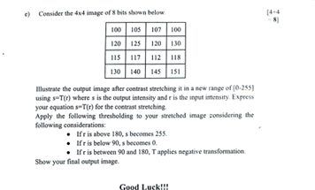
4x4 8-bit image [100 105 107 100; 120 125 120 130; 115 117 112 118; 130 140 145 151]. Illustrate the output after contrast stretching to [0-255] using s=T(r); express s=T(r). Then apply thresholding to the stretched image: r>180 -> 255, r<90 -> 0, 90<=r<=180 -> negative transformation. Show final output image. [4+4]

Worked answer (deck 04)

Same answer as F23 3d (F23 Q3(d) part 1 = SP24 Q3(e) part 1).

SP24 Q3(e) part 24 marks

Apply to the stretched image: r > 180 → 255; r < 90 → 0; 90 ≤ r ≤ 180 → negative transformation. Show the final image.

s =

255

if r > 180

255 − r

if 90 ≤ r ≤ 180

if r < 90

SP24 rule: three pieces. 0 below 90, negative between 90 and 180, 255 above 180.

stretched r	rule	s
0	< 90 → 0	0
25	< 90 → 0	0
35	< 90 → 0	0
60	< 90 → 0	0
75	< 90 → 0	0
85	< 90 → 0	0
90	255 − 90	165
100	255 − 100	155
125	255 − 125	130
150	255 − 150	105
200	> 180 → 255	255
225	> 180 → 255	255
255	> 180 → 255	255

0	25	35	0
100	125	100	150
75	85	60	90
150	200	225	255

stretched r

0	0	0	0
155	130	155	105
0	0	0	165
105	255	255	255

final output

F23 1bCLO1 · Intensity transforms notes · 4

Write short notes on Negative transformation and Intensity level slicing. [2+2]

Worked answer (deck 04)

F23 Q1(b), first half2 marks

Write a short note on the Negative transformation.

The negative transformation is a basic linear intensity transformation that reverses the intensity values of an image (light ↔ dark). For an image with L gray levels in the range [0, L−1]:

s = (L − 1) − r

where r is the input and s the output gray level. Its graph is a straight line from (0, L−1) down to (L−1, 0) [draw it].

Use: enhancing white or gray detail embedded in dark regions, especially when black areas dominate, e.g. medical X-ray and mammogram images.

Example (8-bit): r = 100 gives s = 255 − 100 = 155.

F23 Q1(b), second half2 marks

Write a short note on intensity-level slicing.

Intensity-level (gray-level) slicing highlights a specific range [A, B] of gray levels in an image. It is similar to thresholding, and it is useful when different features of an image lie in different gray levels (e.g. blood vessels in an angiogram).

Two basic approaches: (1) without background: highlight [A, B] and reduce all other levels to a low constant level; (2) with background: highlight [A, B] and preserve all other levels. [Draw both small graphs.]

F23 3dCLO2 · Contrast stretching numeric · 10

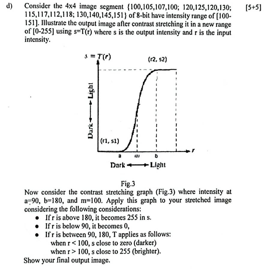
4x4 segment {100,105,107,100; 120,125,120,130; 115,117,112,118; 130,140,145,151}, 8-bit, range [100-151]. Output after contrast stretching to [0-255] using s=T(r). Then apply contrast stretching graph (Fig.3) a=90, b=180, m=100: r>180 -> 255, r<90 -> 0, between: r<100 s near 0, r>100 s near 255. Show final output image. [5+5]

Worked answer (deck 04)

F23 Q3(d) part 1 = SP24 Q3(e) part 15 marks

A 4×4 segment of an 8-bit image has range [100–151]. Find the output after contrast stretching to [0–255] using s = T(r), and express s = T(r).

100	105	107	100
120	125	120	130
115	117	112	118
130	140	145	151

input image

Given: Min = 100, Max = 151, NewMin = 0, NewMax = 255.

Formula: s = (r − Min) × (NewMax − NewMin)/(Max − Min) + NewMin

(NewMax − NewMin)/(Max − Min) = (255 − 0)/(151 − 100) = 255/51 = 5

s = T(r) = 5 (r − 100)

Apply to every gray level:

r	working	s
100	(255 − 0)/(151 − 100) × (100 − 100) + 0 = 5 × 0	0
105	(255 − 0)/(151 − 100) × (105 − 100) + 0 = 5 × 5	25
107	(255 − 0)/(151 − 100) × (107 − 100) + 0 = 5 × 7	35
112	(255 − 0)/(151 − 100) × (112 − 100) + 0 = 5 × 12	60
115	(255 − 0)/(151 − 100) × (115 − 100) + 0 = 5 × 15	75
117	(255 − 0)/(151 − 100) × (117 − 100) + 0 = 5 × 17	85
118	(255 − 0)/(151 − 100) × (118 − 100) + 0 = 5 × 18	90
120	(255 − 0)/(151 − 100) × (120 − 100) + 0 = 5 × 20	100
125	(255 − 0)/(151 − 100) × (125 − 100) + 0 = 5 × 25	125
130	(255 − 0)/(151 − 100) × (130 − 100) + 0 = 5 × 30	150
140	(255 − 0)/(151 − 100) × (140 − 100) + 0 = 5 × 40	200
145	(255 − 0)/(151 − 100) × (145 − 100) + 0 = 5 × 45	225
151	(255 − 0)/(151 − 100) × (151 − 100) + 0 = 5 × 51	255

Output image:

100	105	107	100
120	125	120	130
115	117	112	118
130	140	145	151

input r

0	25	35	0
100	125	100	150
75	85	60	90
150	200	225	255

stretched s

Min-max stretch: the band 100–151 is spread across the whole 0–255.

Check: the old contrast was 151 − 100 = 51; the new contrast is 255 − 0 = 255. Midpoint m = 125 (slide 40).

F23 Q3(d) part 25 marks

Apply the contrast-stretching graph with a = 90, b = 180, m = 100 to the stretched image: r > 180 → 255; r < 90 → 0; between them, r < 100 moves close to 0 and r > 100 moves close to 255. Show the final image.

Slide 42 S-curve: below 90 → 0, above 180 → 255, between them values move away from m.

s =

255

if r > 180

close to 0 (darker)

if 90 ≤ r < 100

close to 255 (brighter)

if 100 < r ≤ 180

if r < 90

Apply to each stretched value (taking the curve at its limit: the dark side goes to 0 and the bright side goes to 255):

stretched r	rule	s
0	< 90	0
25	< 90	0
35	< 90	0
60	< 90	0
75	< 90	0
85	< 90	0
90	90–100, toward 0	0
100	≥ 100, toward 255	255
125	≥ 100, toward 255	255
150	≥ 100, toward 255	255
200	> 180	255
225	> 180	255
255	> 180	255

r = 100 sits exactly at m. I place it on the bright side; write your assumption in the script.

0	25	35	0
100	125	100	150
75	85	60	90
150	200	225	255

stretched r

0	0	0	0
255	255	255	255
0	0	0	0
255	255	255	255

final output

Bright pixels became brighter and dark pixels darker, so the result has higher contrast (here, the limit is a binary image).

SP23 2dCLO1 · Piecewise linear: · 5

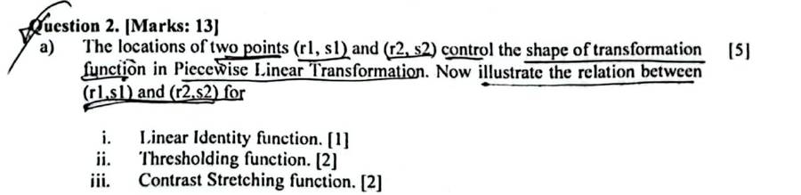
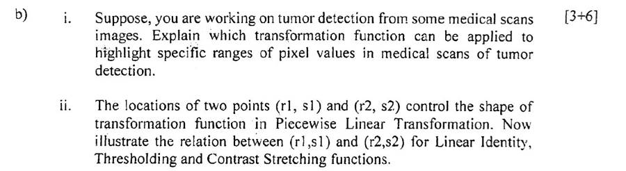
Points A(r1,s1), B(r2,s2) control the piecewise linear transformation. Illustrate the relation between (r1,s1) and (r2,s2) for Linear Identity, Thresholding and Contrast Stretching. [1+2+2]

Worked answer (deck 04)

SP23 2(d) · F22 A1(b)ii · SP22 2(a) · F21 B3(b)5–6 marks, asked 5 times

Points A(r1, s1) and B(r2, s2) control the piecewise linear transformation. Illustrate the relation between (r1, s1) and (r2, s2) for (i) linear identity (ii) thresholding (iii) contrast stretching.

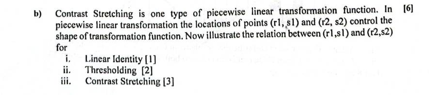
The shape of the piecewise linear function s = T(r) is decided by the two points (r1, s1) and (r2, s2), with r1 ≤ r2 and s1 ≤ s2 so the function stays increasing.

(i) Linear identity: r1 = s1 and r2 = s2. Both points lie on the diagonal, so the line is s = r and the gray levels do not change.

(ii) Thresholding: r1 = r2, s1 = 0, s2 = L−1. The line jumps vertically at r1, so every pixel below r1 becomes 0 and every pixel above becomes L−1: a binary image.

(iii) Contrast stretching: r1 < r2 and s1 < s2. The middle piece between r1 and r2 is steeper than 45°, so those gray levels are spread over a wider output range and contrast increases. Special case, min-max stretching: (r1, s1) = (r_min, 0), (r2, s2) = (r_max, L−1).

(i) Identity: r1 = s1, r2 = s2

(ii) Thresholding: r1 = r2, s1 = 0, s2 = L−1

(iii) Contrast stretching: r1 < r2, s1 < s2

SP22 2aCLO1 · Piecewise linear: · 5

Points (r1,s1),(r2,s2) control the piecewise linear transformation. Illustrate the relation for i) Linear Identity [1] ii) Thresholding [2] iii) Contrast Stretching [2].

Worked answer (deck 04)

Same answer as SP23 2d (SP23 2(d) · F22 A1(b)ii · SP22 2(a) · F21 B3(b)).

F21 B3bCLO1 · Piecewise linear: · 6

Contrast stretching is a piecewise linear transformation; points (r1,s1),(r2,s2). Illustrate the relation for i) Linear Identity [1] ii) Thresholding [2] iii) Contrast Stretching [3].

Worked answer (deck 04)

Same answer as SP23 2d (SP23 2(d) · F22 A1(b)ii · SP22 2(a) · F21 B3(b)).

F25 quiz Q1C 1CLO1 · Intensity transforms notes · 6

Discuss logarithmic transformations for image enhancement. [6]

Worked answer (F25 quiz page)

Fall 25 Quiz 1 (set C) Q16 marks

Discuss logarithmic transformations for image enhancement.

Definition. The log transformation is a basic intensity transformation:

s = c · log(1 + r)

r = input gray level, s = output gray level, c = a constant, r ≥ 0. The 1 is added so that log 0 never occurs. To map 0…255 onto 0…255, c = 255 / log(256) = 105.89.

Shape. Draw this graph in the answer script:

s = c·log(1 + r), c = 105.89 (8-bit). Dashed: identity s = r.

The curve lies above the diagonal. It is steep for small r and flat for large r.

Properties.

For low input values the range is expanded: dark regions are spread out and their details become visible.
For high input values the range is compressed: bright regions are squeezed together.

Worked values (c = 105.89):

r	c·log(1 + r)	s
10	105.89 × log(11) = 110.3	110
50	105.89 × log(51) = 180.8	181
100	105.89 × log(101) = 212.2	212
255	105.89 × log(256) = 255.0	255

The input band 0–50 (20% of the range) becomes 0–181 (71%). The band 100–255 shrinks to 212–255.

Application. Use it when the input has a very large dynamic range that the display cannot show. The standard example is the Fourier spectrum, whose values run from 0 to about 1.5×10⁶. On a display only the bright centre shows; after the log transform the whole spectrum is visible. That is why it is called dynamic-range compression.

Inverse log, s = 10^r/c − 1, does the opposite: it expands the bright values and compresses the dark ones.

Try it: move r and watch where it lands on the curve. Notice how a small step in the dark end moves s a lot, and the same step in the bright end hardly moves it.

F25 quiz Q1C 2aCLO2 · Gray-level · 11

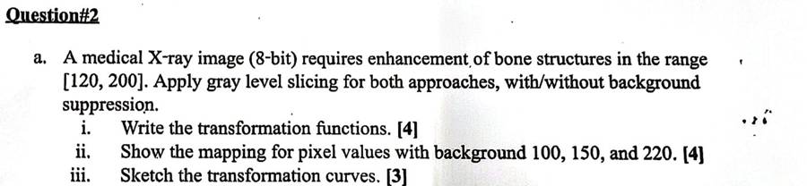
Medical X-ray image (8-bit) needs enhancement of bone structures in range [120, 200]. Apply gray level slicing for both approaches (with/without background suppression). i) Write the transformation functions [4] ii) Show the mapping for pixel values 100, 150 and 220 [4] iii) Sketch the transformation curves [3].

Worked answer (F25 quiz page)

Fall 25 Quiz 2(a)11 marks

A medical X-ray image (8-bit) needs its bone structures in the range [120, 200] enhanced. Apply gray-level slicing with both approaches. (i) Write the transformation functions [4] (ii) Show the mapping for pixel values 100, 150 and 220 [4] (iii) Sketch the transformation curves [3].

Given: 8-bit, so L − 1 = 255. Band of interest A = 120, B = 200. Highlight level = 255.

(i) Transformation functions

Approach 1, without background (other levels suppressed):

s =

255

if 120 ≤ r ≤ 200

otherwise

Approach 2, with background (other levels preserved):

s =

255

if 120 ≤ r ≤ 200

otherwise

(ii) Mapping

r	inside [120, 200]?	Approach 1 s	Approach 2 s
100	no	0	100
150	yes	255	255
220	no	0	220

r = 100 is below the band: approach 1 gives 0, approach 2 keeps 100. r = 150 is inside: both give 255. r = 220 is above: approach 1 gives 0, approach 2 keeps 220.

(iii) Curves

Approach 1: 0, jump to 255 on [120, 200], back to 0.

Approach 2: s = r, lifted to 255 on [120, 200].

Result: approach 1 shows only the bones, white on black. Approach 2 shows the bones in white with the rest of the X-ray still visible.

Try it: type any pixel value, or change the band, and read off both approaches. The dot moves on both curves.

F25 quiz Q1C 2bCLO2 · Resolution / bits / levels arithmetic · 3

How many different shades of grey are possible in a 10-bit grayscale image? Show their numeric range. Illustrate the expression of intensity resolution of any gray image. [3]

Worked answer (F25 quiz page)

Fall 25 Quiz 2(b)3 marks

How many shades of gray are possible in a 10-bit grayscale image? Show the numeric range. Write the expression for intensity resolution.

Intensity resolution = number of gray levels a pixel can take. With k bits per pixel:

L = 2^k

Here k = 10, so L = 2¹⁰ = 1024 shades.

Range: 0 to L − 1 = 0 to 1023 (0 = black, 1023 = white).

Answer1024 gray levels, from 0 to 1023. General expression: L = 2^k, range [0, 2^k − 1].

In plain wordsEvery extra bit doubles the number of grays. 8 bits give 256, 10 bits give 1024, so the steps between neighbouring grays are 4 times finer. Fewer bits give visible bands (false contouring).

Try it: slide k and read off L = 2^k and the range. The strip shows the gray steps, which become visible bands at small k.

More worked examples: slides and other examiners (10)

Slide 12 · Example 1 (deck 04)

Slide 12 · Example 1worked

The matrix gives the pixel values of an 8-bit image r. Apply the negative transform and find the resulting pixel values.

Given: 8-bit image, so L = 2⁸ = 256.

Formula: s = (L − 1) − r = 255 − r. Apply it to every pixel.

r	255 − r	s
85	255 − 85	170
88	255 − 88	167
89	255 − 89	166
90	255 − 90	165
95	255 − 95	160
98	255 − 98	157
99	255 − 99	156
100	255 − 100	155
102	255 − 102	153
105	255 − 105	150
110	255 − 110	145
115	255 − 115	140
135	255 − 135	120
140	255 − 140	115
145	255 − 145	110

100	110	90	95
98	140	145	135
89	90	88	85
102	105	99	115

input image r

155	145	165	160
157	115	110	120
166	165	167	170
153	150	156	140

negative image s

Slide 13 · Exercise (deck 04)

Slide 13 · Exercisesolved

The matrix gives the pixel values of a 5-bit image r. Apply the negative transform.

Given: 5-bit image, so L = 2⁵ = 32 and L − 1 = 31.

Formula: s = 31 − r.

r	31 − r	s
16	31 − 16	15
18	31 − 18	13
19	31 − 19	12
20	31 − 20	11
21	31 − 21	10
23	31 − 23	8
26	31 − 26	5
27	31 − 27	4
29	31 − 29	2
30	31 − 30	1
31	31 − 31	0

21	26	29	30
19	21	20	30
16	16	26	31
19	18	27	23

input r (5-bit)

10	5	2	1
12	10	11	1
15	15	5	0
12	13	4	8

negative s

Mini example (slide 75 image, T = 3) (deck 04)

Mini example (slide 75 image, T = 3)worked

Given: 3-bit image, threshold T = 3. Rule: s = 1 if r > 3, otherwise s = 0.

Values 0, 1, 2, 3 become 0. Values 4, 5, 6, 7 become 1.

2	1	2	1	0
7	1	4	3	2
2	4	1	3	7
1	3	4	6	3
1	4	1	3	4

input r

0	0	0	0	0
1	0	1	0	0
0	1	0	0	1
0	0	1	1	0
0	1	0	0	1

thresholded s

Numeric log example (8-bit) (deck 04)

Numeric log example (8-bit)worked

Choose c so that the top input stays at the top: c = (L−1) / log(1 + (L−1)) = 255 / log₁₀(256) = 255 / 2.4082 = 105.89.

Formula: s = 105.89 × log₁₀(1 + r), then round.

r	1 + r	log₁₀(1+r)	× c	s
0	1	0.0000	0.0	0
1	2	0.3010	31.9	32
5	6	0.7782	82.4	82
10	11	1.0414	110.3	110
50	51	1.7076	180.8	181
100	101	2.0043	212.2	212
200	201	2.3032	243.9	244
255	256	2.4082	255.0	255

Inputs 0–50 went to 0–181 (spread out). Inputs 100–255 went to 212–255 (squeezed). Any log base gives the same s, as long as c uses the same base.

Practice · gamma on a 3-bit image (deck 04)

Practice · gamma on a 3-bit imageworked

The 3×3 image below is transformed using the gamma transformation with γ = 0.5 and γ = 2.0. Find the outputs and discuss the effect of changing γ.

1	4	6
0	2	7
3	5	2

input image

Step 1, find L. The largest value is 7, so the image is 3-bit: L = 8, L − 1 = 7. Take c = 1 on the normalized values.

Step 2, formula. s = 7 × (r/7)^γ, rounded to the nearest integer.

Step 3, one value in full (r = 3, γ = 0.5): 3/7 = 0.4286; 0.4286^0.5 = 0.6547; 7 × 0.6547 = 4.58 → 5.

Step 4, table for every gray level, γ = 0.5:

r	r/7	(r/7)^0.5	×7	s
0	0.0000	0.0000	0.00	0
1	0.1429	0.3780	2.65	3
2	0.2857	0.5345	3.74	4
3	0.4286	0.6547	4.58	5
4	0.5714	0.7559	5.29	5
5	0.7143	0.8452	5.92	6
6	0.8571	0.9258	6.48	6
7	1.0000	1.0000	7.00	7

γ = 2.0:

r	r/7	(r/7)^2.0	×7	s
0	0.0000	0.0000	0.00	0
1	0.1429	0.0204	0.14	0
2	0.2857	0.0816	0.57	1
3	0.4286	0.1837	1.29	1
4	0.5714	0.3265	2.29	2
5	0.7143	0.5102	3.57	4
6	0.8571	0.7347	5.14	5
7	1.0000	1.0000	7.00	7

Step 5, replace each pixel.

1	4	6
0	2	7
3	5	2

input

3	5	6
0	4	7
5	6	4

γ = 0.5

0	2	5
0	1	7
1	4	1

γ = 2.0

Practice mapping drawn: γ = 0.5 points sit above the diagonal, γ = 2.0 below.

Step 6, effect of γ.

γ = 0.5 (< 1) pushes values up: the image becomes brighter. Dark levels 1–3 are spread to 3–5 (more detail in dark areas); bright levels 4–7 bunch at 5–7.
γ = 2.0 (> 1) pushes values down: the image becomes darker. Levels 0–1 collapse to 0 and 2–3 to 1; bright levels 5–7 are spread to 4–7 (more detail in bright areas).
So a smaller γ brightens and gives contrast to dark regions; a larger γ darkens and gives contrast to bright regions. γ = 1 leaves the image unchanged.

Short note (deck 04)

Short notetheory

Many devices (image capture, printing, display) respond to intensity according to a power law, so they need to be corrected. A CRT monitor has an intensity-to-voltage response with exponent about 1.8 to 2.5, so images look darker than they should.
Gamma correction is the process used to correct this power-law response: pre-process the image with s = c·r^1/2.5 so the monitor's darkening cancels out.
Background: human vision is nonlinear (more sensitive to small changes in dark tones than bright ones), while digital sensors are linear.
Different display devices have different gammas, so each needs its own correction.
Why needed: to display an image accurately on screen (without correction it looks bleached out or, more likely, too dark); to reproduce colours accurately; and for general-purpose contrast manipulation.

Slides 60–61 · 3-bit example (deck 04)

Slides 60–61 · 3-bit exampleworked

Step 1. Write each pixel of the 3-bit image in binary.

6	7	6	6	7
0	0	0	1	2
1	1	1	2	3
4	5	5	4	2
6	6	6	7	7

3-bit image

110	111	110	110	111
000	000	000	001	010
001	001	001	010	011
100	101	101	100	010
110	110	110	111	111

binary

Step 2. Collect the 1st bit of every pixel (MSB plane), the 2nd bit (centre plane), and the 3rd bit (LSB plane).

1	1	1	1	1
0	0	0	0	0
0	0	0	0	0
1	1	1	1	0
1	1	1	1	1

MSB plane (×4)

1	1	1	1	1
0	0	0	0	1
0	0	0	1	1
0	0	0	0	1
1	1	1	1	1

centre plane (×2)

0	1	0	0	1
0	0	0	1	0
1	1	1	0	1
0	1	1	0	0
0	0	0	1	1

LSB plane (×1)

Check one pixel: 6 = 110 gives MSB 1, centre 1, LSB 0.

Slides 63–67 (deck 04)

Slides 63–67worked

Given: A = [167 133 111; 144 140 135; 159 154 148] and its bit format:

10100111	10000101	01101111
10010000	10001100	10000111
10011111	10011010	10010100

A in binary

8th plane only. For 10100111, multiply only the 8th bit by 2⁷ = 128: (1×128) + (0×0) + (1×0) + (0×0) + (0×0) + (1×0) + (1×0) + (1×0) = 128. 111 = 01101111 has 8th bit 0, so it gives 0.

Bitwise AND view (slides 64–65): pixel AND 10000000 (128) keeps the 8th bit only; pixel AND 01000000 (64) keeps the 7th bit only.

128	128	0
128	128	128
128	128	128

8th plane image

0	0	64
0	0	0
0	0	0

7th plane image

128	128	64
128	128	128
128	128	128

8th + 7th planes

8th + 7th combined (slide 66): for 10100111, (1×128) + (0×64) = 128. For 01101111, (0×128) + (1×64) = 64.

Plane 1 (LSB) and plane 8 (MSB) as 0/1 images (slides 71–72):

1	1	1
0	0	1
1	0	0

plane 1 (LSB)

1	1	0
1	1	1
1	1	1

plane 8 (MSB)

Slide 74 · Exercise (deck 04)

Slide 74 · Exercisesolved

Using the same A, reconstruct the image using only (a) the 5th and 4th bit planes (b) the 7th and 6th bit planes.

(a) weights 2⁴ = 16 and 2³ = 8. Example 01101111 (111): 5th bit 0, 4th bit 1, so 0 + 8 = 8. Example 10011111 (159): 16 + 8 = 24.

(b) weights 2⁶ = 64 and 2⁵ = 32. Example 01101111: 64 + 32 = 96. Example 10100111 (167): 0 + 32 = 32.

0	0	8
16	8	0
24	24	16

(a) 5th + 4th

32	0	96
0	0	0
0	0	0

(b) 7th + 6th

(a) is dark and noisy-looking because the low planes hold little of the picture; (b) keeps more structure.

Slide 75 · Class work (deck 04)

Slide 75 · Class workall parts

Apply these enhancement techniques to the 3-bit image I: digital negative; bit planes; thresholding with T = 3; intensity slicing with both approaches, a = 3, b = 5, raising the level to 5. Show the enhanced images.

2	1	2	1	0
7	1	4	3	2
2	4	1	3	7
1	3	4	6	3
1	4	1	3	4

I (3-bit)

Given: 3 bits per pixel, so L = 8 and L − 1 = 7.

(1) Digital negative. s = (L − 1) − r = 7 − r. 0→7, 1→6, 2→5, 3→4, 4→3, 6→1, 7→0.

5	6	5	6	7
0	6	3	4	5
5	3	6	4	0
6	4	3	1	4
6	3	6	4	3

negative

(2) Bit planes. Binary: 0 = 000, 1 = 001, 2 = 010, 3 = 011, 4 = 100, 6 = 110, 7 = 111.

0	0	0	0	0
1	0	1	0	0
0	1	0	0	1
0	0	1	1	0
0	1	0	0	1

plane 2 (MSB, ×4)

1	0	1	0	0
1	0	0	1	1
1	0	0	1	1
0	1	0	1	1
0	0	0	1	0

plane 1 (×2)

0	1	0	1	0
1	1	0	1	0
0	0	1	1	1
1	1	0	0	1
1	0	1	1	0

plane 0 (LSB, ×1)

Check: 4·b2 + 2·b1 + b0 rebuilds I (e.g. 6 → 1, 1, 0 → 4 + 2 = 6).

(3) Thresholding, T = 3.

s =

if r > 3

if r ≤ 3

0	0	0	0	0
1	0	1	0	0
0	1	0	0	1
0	0	1	1	0
0	1	0	0	1

thresholded

Note: this equals the MSB plane, because r > 3 exactly when the first bit is 1.

(4) Intensity slicing, [a, b] = [3, 5], highlight level 5.

Approach 1: s =

if 3 ≤ r ≤ 5

otherwise

Approach 2: s =

if 3 ≤ r ≤ 5

otherwise

0	0	0	0
0	5	5	0
5	0	5	0
5	5	0	5
5	0	5	5

without background

2	1	2	1	0
7	1	5	5	2
2	5	1	5	7
1	5	5	6	5
1	5	1	5	5

with background

Approach 1

Approach 2

3. Histogram: types, equalization, matching

deck 05 · 15 past questions

The pattern: how she asks it

Q2(a), 8 marks, nearly every paper: a 3-bit 5×5 grid or a table of counts. Write PDF, CDF, s = round(7·CDF), then the new histogram, and draw both.
Q1: the 4 histogram types (dark, bright, low, high contrast), whether two images can have the same histogram, the definition and steps of HE.
Rare: histogram matching (F22 A3b uses the slide 49 counts).

Connects to: HE is the automatic version of contrast stretching (ch 3). Its output flattens the histogram, which helps the thresholding and segmentation steps later.

type	CLO	times	where
Histogram equalization	CLO2	9	SP25 2a, SP24 2a, F23 2a, SP23 3b, F22 A3b, SP22 2b, F21 B3a, F25 quiz Q1D 2b, F25 quiz Q2C 2
Histogram concepts	CLO1	6	F23 1a, SP23 2b, F22 A2b, F25 quiz Q1D 1, F25 quiz Q1D 2a, F25 quiz Q2C 1
Histogram equalization definition / steps / effect	CLO1	1	F22 A2b

Formula wall: every formula with a worked line

p(r_k) = n_k / N → CDF = Σ p → s_k = round( (L−1) × CDF_k )

Worked (3-bit, N = 64, n_k = [8, 10, 10, 2, 12, 16, 4, 2]). Do every row like the first two:

r = 0: p = 8/64 = 0.125, CDF = 0.125, 7 × 0.125 = 0.875 → 1. r = 1: p = 10/64 = 0.15625, CDF = 0.28125, 7 × 0.28125 = 1.969 → 2.

r	n_k	p	CDF	7 × CDF	s
0	8	0.1250	0.1250	0.875	1
1	10	0.1562	0.2812	1.969	2
2	10	0.1562	0.4375	3.062	3
3	2	0.0312	0.4688	3.281	3
4	12	0.1875	0.6562	4.594	5
5	16	0.2500	0.9062	6.344	6
6	4	0.0625	0.9688	6.781	7
7	2	0.0312	1.0000	7.000	7

New histogram: add the counts that land on the same s: s = 3 gets 10 + 2 = 12; s = 7 gets 4 + 2 = 6. Total stays 64.

Equalized histogram: spread out, not perfectly flat, because levels are discrete. Write that sentence.

Matching (if asked): equalize the input → H, equalize the target → S, map each r to the z whose S is closest to its H (ties → higher S).

TrapDraw three things: the original histogram, the equalized histogram and the transformation (staircase). Each is a separate mark.

Past questions: look, recall, then open the answer

SP25 2aCLO2 · Histogram equalization · 8

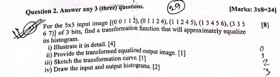
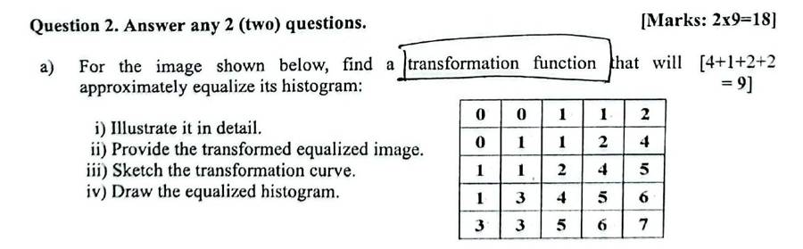
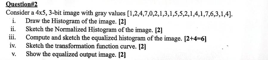
For the 5x5 input image [(0 0 1 1 2),(0 1 1 2 4),(1 1 2 4 5),(1 3 4 5 6),(3 3 5 6 7)] of 3 bits, find a transformation function that will approximately equalize its histogram. i) Illustrate it in detail [4] ii) Provide the transformed equalized output image [1] iii) Sketch the transformation curve [1] iv) Draw the input and output histograms [2].

Worked answer (deck 05)

SP25 Q2(a) · SP24 Q2(a)8–9 marks

For the 5×5, 3-bit input image, find a transformation function that will approximately equalize its histogram. (i) Illustrate in detail (ii) give the equalized output image (iii) sketch the transformation curve (iv) draw the input and output histograms.

Given: 3-bit image, so L = 2³ = 8 and L − 1 = 7. Total pixels N = 25.

0	0	1	1	2
0	1	1	2	4
1	1	2	4	5
1	3	4	5	6
3	3	5	6	7

input image

Step 1, histogram h(r_k) = n_k: count the pixels at each gray level.

r_k	0	1	2	3	4	5	6	7
n_k	3	7	3	3	3	3	2	1

Check: Σ n_k = 3 + 7 + 3 + 3 + 3 + 3 + 2 + 1 = 25.

_kn_k

Original histogram (n_k against r_k)

_kp(r_k)

Normalized histogram p(r_k) = n_k/N

Steps 2–5. PDF p(r_k) = n_k/N; CDF = running sum of the PDF; multiply by (L − 1) = 7; round off (.5 goes up).

r_k	Step 1: n_k	Step 2: PDF	Step 3: CDF	Step 4: (L−1)·CDF	Step 5: s_k
0	3	0.1200	0.1200	7 × 0.1200 = 0.8400	1
1	7	0.2800	0.4000	7 × 0.4000 = 2.8000	3
2	3	0.1200	0.5200	7 × 0.5200 = 3.6400	4
3	3	0.1200	0.6400	7 × 0.6400 = 4.4800	4
4	3	0.1200	0.7600	7 × 0.7600 = 5.3200	5
5	3	0.1200	0.8800	7 × 0.8800 = 6.1600	6
6	2	0.0800	0.9600	7 × 0.9600 = 6.7200	7
7	1	0.0400	1.0000	7 × 1.0000 = 7.0000	7

Mapping the new gray levels into number of pixels:

gray level r_k	new gray level s_k	no. of pixels n_k
0	1	3
1	3	7
2	4	3
3	4	3
4	5	3
5	6	3
6	7	2
7	7	1

Equalized histogram: add the n_k that land on the same s_k. Levels not listed get 0 pixels.

s_k	pixels added	n(s_k)
1	3	3
3	7	7
4	3 + 3 = 6	6
5	3	3
6	3	3
7	2 + 1 = 3	3

_kn_k

Equalized histogram (n against new level s_k)

_koutput s_k

Transformation function s_k = T(r_k) drawn as a staircase (slide 40 style). Empty levels keep the previous step.

Equalized output image: replace every pixel r by its s.

0	0	1	1	2
0	1	1	2	4
1	1	2	4	5
1	3	4	5	6
3	3	5	6	7

input

1	1	3	3	4
1	3	3	4	5
3	3	4	5	6
3	4	5	6	7
4	4	6	7	7

equalized output

Try it, step by step: SP25 / SP24, every step.

SP24 2aCLO2 · Histogram equalization · 9

For the 5x5 image [(0 0 1 1 2),(0 1 1 2 4),(1 1 2 4 5),(1 3 4 5 6),(3 3 5 6 7)] find a transformation function that will approximately equalize its histogram: i) illustrate in detail ii) transformed equalized image iii) sketch transformation curve iv) draw equalized histogram [4+1+2+2]

Worked answer (deck 05)

Same answer as SP25 2a (SP25 Q2(a) · SP24 Q2(a)).

F23 1aCLO1 · Histogram concepts · 4

What is the histogram of an image? Can you reconstruct the image from the histogram? How does the histogram differ for dark, bright, low contrast or high contrast image? [1+1+2]

Worked answer (deck 05)

F23 Q1(a)4 marks

What is the histogram of an image? Can you reconstruct the image from the histogram? How does the histogram differ for a dark, bright, low-contrast or high-contrast image? [1+1+2]

Histogram: a graphical representation of the distribution of pixel intensity values in an image. For gray levels in [0, L−1] it is the discrete function h(r_k) = n_k, where n_k is the number of pixels with gray level r_k.

Reconstruction: No. A histogram holds only statistical information (how many pixels have each value), not the location of the pixels. Different images can have the same histogram, e.g. a half-black/half-white image and a checkerboard with the same numbers of black and white pixels.

Four types [draw the four small histograms]:

dark

bright

low contrast

high contrast

Dark: components concentrated on the low (left) side of the gray scale.
Bright: concentrated on the high (right) side.
Low contrast: a narrow band, usually in the middle of the scale.
High contrast: spread over a broad range, fairly uniformly.

F23 2aCLO2 · Histogram equalization · 6

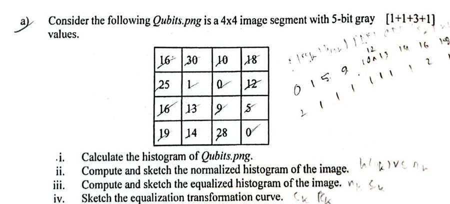
Qubits.png 4x4, 5-bit: [[16,30,10,18],[25,1,0,12],[16,13,9,5],[19,14,28,0]]. i) histogram ii) compute and sketch normalized histogram iii) compute and sketch equalized histogram iv) sketch equalization transformation curve [1+1+3+1]

Worked answer (deck 05)

F23 Q2(a) · Qubits.png6 marks

4×4, 5-bit image. (i) histogram (ii) compute and sketch the normalized histogram (iii) compute and sketch the equalized histogram (iv) sketch the transformation curve.

Given: 5-bit image, so L = 2⁵ = 32 and L − 1 = 31. Total pixels N = 16.

16	30	10	18
25	1	0	12
16	13	9	5
19	14	28	0

input image

Step 1, histogram h(r_k) = n_k: count the pixels at each gray level.

r_k	0	1	2	3	4	5	6	7	8	9	10	11	12	13	14	15	16	17	18	19	20	21	22	23	24	25	26	27	28	29	30	31
n_k	2	1	0	0	0	1	0	0	0	1	1	0	1	1	1	0	2	0	1	1	0	0	0	0	0	1	0	0	1	0	1	0

Check: Σ n_k = 2 + 1 + 1 + 1 + 1 + 1 + 1 + 1 + 2 + 1 + 1 + 1 + 1 + 1 = 16.

_kn_k

Original histogram (n_k against r_k)

_kp(r_k)

Normalized histogram p(r_k) = n_k/N

Steps 2–5. PDF p(r_k) = n_k/N; CDF = running sum of the PDF; multiply by (L − 1) = 31; round off (.5 goes up). Only the intensities with non-zero occurrence are listed, as the slide says.

r_k	Step 1: n_k	Step 2: PDF	Step 3: CDF	Step 4: (L−1)·CDF	Step 5: s_k
0	2	0.1250	0.1250	31 × 0.1250 = 3.8750	4
1	1	0.0625	0.1875	31 × 0.1875 = 5.8125	6
5	1	0.0625	0.2500	31 × 0.2500 = 7.7500	8
9	1	0.0625	0.3125	31 × 0.3125 = 9.6875	10
10	1	0.0625	0.3750	31 × 0.3750 = 11.6250	12
12	1	0.0625	0.4375	31 × 0.4375 = 13.5625	14
13	1	0.0625	0.5000	31 × 0.5000 = 15.5000	16
14	1	0.0625	0.5625	31 × 0.5625 = 17.4375	17
16	2	0.1250	0.6875	31 × 0.6875 = 21.3125	21
18	1	0.0625	0.7500	31 × 0.7500 = 23.2500	23
19	1	0.0625	0.8125	31 × 0.8125 = 25.1875	25
25	1	0.0625	0.8750	31 × 0.8750 = 27.1250	27
28	1	0.0625	0.9375	31 × 0.9375 = 29.0625	29
30	1	0.0625	1.0000	31 × 1.0000 = 31.0000	31

Mapping the new gray levels into number of pixels:

gray level r_k	new gray level s_k	no. of pixels n_k
0	4	2
1	6	1
5	8	1
9	10	1
10	12	1
12	14	1
13	16	1
14	17	1
16	21	2
18	23	1
19	25	1
25	27	1
28	29	1
30	31	1

Equalized histogram: add the n_k that land on the same s_k. Levels not listed get 0 pixels.

s_k	pixels added	n(s_k)
4	2	2
6	1	1
8	1	1
10	1	1
12	1	1
14	1	1
16	1	1
17	1	1
21	2	2
23	1	1
25	1	1
27	1	1
29	1	1
31	1	1

_kn_k

Equalized histogram (n against new level s_k)

_koutput s_k

Transformation function s_k = T(r_k) drawn as a staircase (slide 40 style). Empty levels keep the previous step.

Equalized output image: replace every pixel r by its s.

16	30	10	18
25	1	0	12
16	13	9	5
19	14	28	0

input

21	31	12	23
27	6	4	14
21	16	10	8
25	17	29	4

equalized output

Try it, step by step: F23 (5-bit): only the levels that occur get a table row.

SP23 2bCLO1 · Histogram concepts · 5

What is histogram of an image? Write the four basic intensity characteristics of image and their corresponding histograms. [1+2+2]

Worked answer (deck 05)

SP23 Q2(b) · Fall 25 Quiz (D) Q2(a)4–5 marks

What is the histogram of an image? Explain the four basic intensity characteristics of an image and their corresponding histograms.

Write the definition and h(r_k) = n_k as above, then the four types with their four sketches. Add the meaning of each:

Dark image: most pixels have low values, so the histogram sits on the left; the image looks dark and details in shadows are hidden.
Bright image: most pixels have high values, so the histogram sits on the right; the image looks washed out.
Low-contrast image: pixels occupy a narrow range of gray levels, so the histogram is narrow; the image looks dull and gray.
High-contrast image: pixels cover almost the whole range and the histogram is spread fairly evenly; the image shows a lot of gray-level detail.

SP23 3bCLO2 · Histogram equalization · 8

4x4 image, 4-bit gray values [1,2,4,7,2,1,3,1,5,2,1,4] (only 12 printed; student wrote 7,6,3,1). i) Compute and sketch histogram and normalized histogram ii) equalized histogram iii) equalization transformation function. [3+3+2]

Worked answer (F25 quiz page)

SP23 Q3(b)8 marks

4-bit image, so L = 16 and the levels are 0 to 15. MN = 16. The last row (7 6 3 1) is how the student copy reads.

i) Histogram and normalized histogram: count each level, p(r_k) = n_k/16.

histogram h(r_k) = n_k (levels 9–15 are 0)

iii) Transformation s_k = round(15 · CDF), .5 rounds up:

r_k	n_k	p(r_k)	CDF	15 · CDF	s_k
1	5	5/16 = 0.3125	5/16 = 0.3125	15 × 0.3125 = 4.6875	5
2	3	3/16 = 0.1875	8/16 = 0.5000	15 × 0.5000 = 7.5000	8
3	2	2/16 = 0.1250	10/16 = 0.6250	15 × 0.6250 = 9.3750	9
4	2	2/16 = 0.1250	12/16 = 0.7500	15 × 0.7500 = 11.2500	11
5	1	1/16 = 0.0625	13/16 = 0.8125	15 × 0.8125 = 12.1875	12
6	1	1/16 = 0.0625	14/16 = 0.8750	15 × 0.8750 = 13.1250	13
7	2	2/16 = 0.1250	16/16 = 1.0000	15 × 1.0000 = 15.0000	15

ii) Equalized histogram: move each count to its new level s_k.

equalized histogram: the counts now spread from 5 to 15

Mapping: 1→5, 2→8, 3→9, 4→11, 5→12, 6→13, 7→15. The levels spread over the whole 0–15 range, so contrast goes up.

Try it, step by step: the same 4-bit image, step by step.

F22 A2bCLO1 · Histogram concepts · 3CLO1 · Histogram equalization definition / steps / effect · 2

What is histogram of an image? How does the histogram differ for dark, bright, low contrast, high contrast image of the same scene? Write the steps of histogram equalization algorithm. [1+2+2]

Worked answer (deck 05)

F22 A2(b)5 marks

What is the histogram of an image? How does the histogram differ for dark, bright, low-contrast and high-contrast images of the same scene? Write the steps of the histogram equalization algorithm. [1+2+2]

Definition and four types as above. Algorithm (input: image f with L levels):

Compute the histogram h(r_k) = n_k.
Compute the PDF p(r_k) = n_k/N.
Compute the CDF, the cumulative sum of the PDF.
Compute s_k = (L − 1) × CDF(r_k).
Round s_k to get the new intensity values, and replace every r_k by s_k.

F22 A3bCLO2 · Histogram equalization · 8

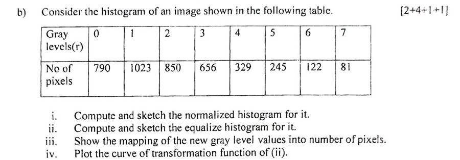
Histogram table r=0..7, n=[790,1023,850,656,329,245,122,81]. i) compute/sketch normalized histogram ii) compute/sketch equalized histogram iii) mapping of new gray levels into number of pixels iv) plot transformation curve. [2+4+1+1]

Worked answer (deck 05)

F22 A3(b) · same counts as slide 498 marks

Histogram r = 0..7, n = [790, 1023, 850, 656, 329, 245, 122, 81]. (i) normalized histogram (ii) equalized histogram (iii) mapping of new gray levels into number of pixels (iv) transformation curve.

Here, as on slide 49, the PDF is rounded to 2 decimal places before the CDF.

Given: 3-bit image, so L = 2³ = 8 and L − 1 = 7. Total pixels N = 4096.

Step 1, histogram h(r_k) = n_k: count the pixels at each gray level.

r_k	0	1	2	3	4	5	6	7
n_k	790	1023	850	656	329	245	122	81

Check: Σ n_k = 790 + 1023 + 850 + 656 + 329 + 245 + 122 + 81 = 4096.

_kn_k

Original histogram (n_k against r_k)

_kp(r_k)

Normalized histogram p(r_k) = n_k/N

Steps 2–5. PDF p(r_k) = n_k/N; CDF = running sum of the PDF; multiply by (L − 1) = 7; round off (.5 goes up).

r_k	Step 1: n_k	Step 2: PDF	Step 3: CDF	Step 4: (L−1)·CDF	Step 5: s_k
0	790	0.19	0.19	7 × 0.19 = 1.33	1
1	1023	0.25	0.44	7 × 0.44 = 3.08	3
2	850	0.21	0.65	7 × 0.65 = 4.55	5
3	656	0.16	0.81	7 × 0.81 = 5.67	6
4	329	0.08	0.89	7 × 0.89 = 6.23	6
5	245	0.06	0.95	7 × 0.95 = 6.65	7
6	122	0.03	0.98	7 × 0.98 = 6.86	7
7	81	0.02	1.00	7 × 1.00 = 7.00	7

Mapping the new gray levels into number of pixels:

gray level r_k	new gray level s_k	no. of pixels n_k
0	1	790
1	3	1023
2	5	850
3	6	656
4	6	329
5	7	245
6	7	122
7	7	81

Equalized histogram: add the n_k that land on the same s_k. Levels not listed get 0 pixels.

s_k	pixels added	n(s_k)
1	790	790
3	1023	1023
5	850	850
6	656 + 329 = 985	985
7	245 + 122 + 81 = 448	448

_kn_k

Equalized histogram (n against new level s_k)

_koutput s_k

Transformation function s_k = T(r_k) drawn as a staircase (slide 40 style). Empty levels keep the previous step.

Try it, step by step: F22 with the PDF rounded to 2 places, as on slide 49.

SP22 2bCLO2 · Histogram equalization · 8

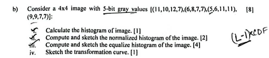
4x4 image, 5-bit [(11,10,12,7),(6,8,7,7),(5,6,11,11),(9,9,7,7)]. i) histogram [1] ii) normalized histogram [2] iii) equalized histogram [4] iv) transformation curve [1].

Worked answer (deck 05)

SP22 Q2(b)8 marks

4×4, 5-bit image. (i) histogram (ii) normalized histogram (iii) equalized histogram (iv) transformation curve.

Given: 5-bit image, so L = 2⁵ = 32 and L − 1 = 31. Total pixels N = 16.

11	10	12	7
6	8	7	7
5	6	11	11
9	9	7	7

input image

Step 1, histogram h(r_k) = n_k: count the pixels at each gray level.

r_k	0	1	2	3	4	5	6	7	8	9	10	11	12	13	14	15	16	17	18	19	20	21	22	23	24	25	26	27	28	29	30	31
n_k	0	0	0	0	0	1	2	5	1	2	1	3	1	0	0	0	0	0	0	0	0	0	0	0	0	0	0	0	0	0	0	0

Check: Σ n_k = 1 + 2 + 5 + 1 + 2 + 1 + 3 + 1 = 16.

_kn_k

Original histogram (n_k against r_k)

_kp(r_k)

Normalized histogram p(r_k) = n_k/N

Steps 2–5. PDF p(r_k) = n_k/N; CDF = running sum of the PDF; multiply by (L − 1) = 31; round off (.5 goes up). Only the intensities with non-zero occurrence are listed, as the slide says.

r_k	Step 1: n_k	Step 2: PDF	Step 3: CDF	Step 4: (L−1)·CDF	Step 5: s_k
5	1	0.0625	0.0625	31 × 0.0625 = 1.9375	2
6	2	0.1250	0.1875	31 × 0.1875 = 5.8125	6
7	5	0.3125	0.5000	31 × 0.5000 = 15.5000	16
8	1	0.0625	0.5625	31 × 0.5625 = 17.4375	17
9	2	0.1250	0.6875	31 × 0.6875 = 21.3125	21
10	1	0.0625	0.7500	31 × 0.7500 = 23.2500	23
11	3	0.1875	0.9375	31 × 0.9375 = 29.0625	29
12	1	0.0625	1.0000	31 × 1.0000 = 31.0000	31

Mapping the new gray levels into number of pixels:

gray level r_k	new gray level s_k	no. of pixels n_k
5	2	1
6	6	2
7	16	5
8	17	1
9	21	2
10	23	1
11	29	3
12	31	1

Equalized histogram: add the n_k that land on the same s_k. Levels not listed get 0 pixels.

s_k	pixels added	n(s_k)
2	1	1
6	2	2
16	5	5
17	1	1
21	2	2
23	1	1
29	3	3
31	1	1

_kn_k

Equalized histogram (n against new level s_k)

_koutput s_k

Transformation function s_k = T(r_k) drawn as a staircase (slide 40 style). Empty levels keep the previous step.

Equalized output image: replace every pixel r by its s.

11	10	12	7
6	8	7	7
5	6	11	11
9	9	7	7

input

29	23	31	16
6	17	16	16
2	6	29	29
21	21	16	16

equalized output

Try it, step by step: SP22 (5-bit), every step.

F21 B3aCLO2 · Histogram equalization · 8

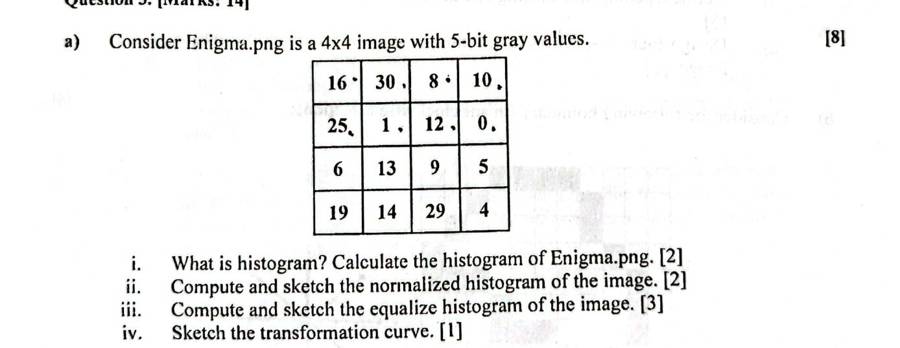
Enigma.png 4x4 5-bit [[16,30,8,10],[25,1,12,0],[6,13,9,5],[19,14,29,4]]. i) What is histogram? Calculate histogram [2] ii) normalized histogram [2] iii) equalized histogram [3] iv) transformation curve [1].

Worked answer (deck 05)

F21 B3(a) · Enigma.png8 marks

(i) What is a histogram? Calculate it. (ii) normalized histogram (iii) equalized histogram (iv) transformation curve. 4×4, 5-bit image.

Histogram: a graphical representation of the distribution of pixel intensity values, h(r_k) = n_k.

Given: 5-bit image, so L = 2⁵ = 32 and L − 1 = 31. Total pixels N = 16.

16	30	8	10
25	1	12	0
6	13	9	5
19	14	29	4

input image

Step 1, histogram h(r_k) = n_k: count the pixels at each gray level.

r_k	0	1	2	3	4	5	6	7	8	9	10	11	12	13	14	15	16	17	18	19	20	21	22	23	24	25	26	27	28	29	30	31
n_k	1	1	0	0	1	1	1	0	1	1	1	0	1	1	1	0	1	0	0	1	0	0	0	0	0	1	0	0	0	1	1	0

Check: Σ n_k = 1 + 1 + 1 + 1 + 1 + 1 + 1 + 1 + 1 + 1 + 1 + 1 + 1 + 1 + 1 + 1 = 16.

_kn_k

Original histogram (n_k against r_k)

_kp(r_k)

Normalized histogram p(r_k) = n_k/N

Steps 2–5. PDF p(r_k) = n_k/N; CDF = running sum of the PDF; multiply by (L − 1) = 31; round off (.5 goes up). Only the intensities with non-zero occurrence are listed, as the slide says.

r_k	Step 1: n_k	Step 2: PDF	Step 3: CDF	Step 4: (L−1)·CDF	Step 5: s_k
0	1	0.0625	0.0625	31 × 0.0625 = 1.9375	2
1	1	0.0625	0.1250	31 × 0.1250 = 3.8750	4
4	1	0.0625	0.1875	31 × 0.1875 = 5.8125	6
5	1	0.0625	0.2500	31 × 0.2500 = 7.7500	8
6	1	0.0625	0.3125	31 × 0.3125 = 9.6875	10
8	1	0.0625	0.3750	31 × 0.3750 = 11.6250	12
9	1	0.0625	0.4375	31 × 0.4375 = 13.5625	14
10	1	0.0625	0.5000	31 × 0.5000 = 15.5000	16
12	1	0.0625	0.5625	31 × 0.5625 = 17.4375	17
13	1	0.0625	0.6250	31 × 0.6250 = 19.3750	19
14	1	0.0625	0.6875	31 × 0.6875 = 21.3125	21
16	1	0.0625	0.7500	31 × 0.7500 = 23.2500	23
19	1	0.0625	0.8125	31 × 0.8125 = 25.1875	25
25	1	0.0625	0.8750	31 × 0.8750 = 27.1250	27
29	1	0.0625	0.9375	31 × 0.9375 = 29.0625	29
30	1	0.0625	1.0000	31 × 1.0000 = 31.0000	31

Mapping the new gray levels into number of pixels:

gray level r_k	new gray level s_k	no. of pixels n_k
0	2	1
1	4	1
4	6	1
5	8	1
6	10	1
8	12	1
9	14	1
10	16	1
12	17	1
13	19	1
14	21	1
16	23	1
19	25	1
25	27	1
29	29	1
30	31	1

Equalized histogram: add the n_k that land on the same s_k. Levels not listed get 0 pixels.

s_k	pixels added	n(s_k)
2	1	1
4	1	1
6	1	1
8	1	1
10	1	1
12	1	1
14	1	1
16	1	1
17	1	1
19	1	1
21	1	1
23	1	1
25	1	1
27	1	1
29	1	1
31	1	1

_kn_k

Equalized histogram (n against new level s_k)

_koutput s_k

Transformation function s_k = T(r_k) drawn as a staircase (slide 40 style). Empty levels keep the previous step.

Equalized output image: replace every pixel r by its s.

16	30	8	10
25	1	12	0
6	13	9	5
19	14	29	4

input

23	31	12	16
27	4	17	2
10	19	14	8
25	21	29	6

equalized output

Try it, step by step: F21 (5-bit), every step.

F25 quiz Q1D 1CLO1 · Histogram concepts · 6

How to generate an image Histogram? What does an image Histogram say? [3+3=6]

Worked answer (F25 quiz page)

Fall 25 Quiz (set D) Q16 marks

How do you generate an image histogram? What does an image histogram say? [3+3]

Generate: (1) find the number of gray levels L = 2^k and make one bin per level 0 … L−1; (2) scan the image and, for each pixel with value r_k, add 1 to bin h(r_k); (3) plot n_k against r_k as bars. Σ h = total number of pixels.

Example (slide 7, 3-bit 4×4): h = [1, 1, 3, 5, 1, 2, 1, 2].

_kn_k

h(r_k) for the slide 7 image

What it says: how many pixels have each intensity, i.e. the tonal distribution. From its shape we can tell whether the image is dark, bright, low- or high-contrast; judge the overall quality and the possibility of enhancement; check whether the image was scanned properly; and choose a threshold for object detection and segmentation. It gives only statistical information and no indication of pixel locations.

Try it: pick an image type. The page makes a small image of that type and counts its histogram from scratch, the same way as in steps 1–3.

F25 quiz Q1D 2aCLO1 · Histogram concepts · 4

Explain the four basic types of intensity characteristics of an image and their corresponding histograms. [4]

Worked answer (F25 quiz page)

Fall 25 Quiz 1 (set D) Q2(a) · also SP23 Q2(b)4 marks

Explain the four basic types of intensity characteristics of an image and their corresponding histograms.

The histogram of a digital image with gray levels 0 … L−1 is h(r_k) = n_k, the number of pixels with gray level r_k. Its shape shows the four basic types:

(1) Dark image

(2) Bright image

(3) Low-contrast image

(4) High-contrast image

Dark image: most pixels have low values, so the histogram is crowded on the left (dark) side. The image looks dark and details in the shadows are hidden.
Bright image: most pixels have high values, so the histogram is crowded on the right side. The image looks washed out.
Low-contrast image: the pixels occupy a narrow range of gray levels in the middle, so the histogram is narrow. The image looks dull and grayish.
High-contrast image: the pixels cover almost the whole range, and the histogram is spread fairly evenly. The image shows a lot of gray-level detail and looks sharp.

Histogram equalization tries to turn types 1–3 into type 4.

Try it: click each type: a fresh random image of that kind and its counted histogram. Compare with the four sketches.

F25 quiz Q1D 2bCLO2 · Histogram equalization · 10

3-bit 8x8 image, histogram counts {0:2, 1:3, 2:5, 3:6, 4:9, 5:12, 6:14, 7:13}. i) Sketch normalized histogram [2] ii) Compute and sketch the equalized histogram [2+4=6] iii) Sketch the transformation function curve [2].

Worked answer (F25 quiz page)

Fall 25 Quiz (set D) Q2(b)10 marks

A 3-bit 8×8 image has histogram counts {{0:2, 1:3, 2:5, 3:6, 4:9, 5:12, 6:14, 7:13}}. (i) Sketch the normalized histogram (ii) compute and sketch the equalized histogram (iii) sketch the transformation function curve.

Given: 3-bit image, so L = 2³ = 8 and L − 1 = 7. Total pixels N = 64.

Step 1, histogram h(r_k) = n_k: count the pixels at each gray level.

r_k	0	1	2	3	4	5	6	7
n_k	2	3	5	6	9	12	14	13

Check: Σ n_k = 2 + 3 + 5 + 6 + 9 + 12 + 14 + 13 = 64.

_kn_k

Original histogram (n_k against r_k)

_kp(r_k)

Normalized histogram p(r_k) = n_k/N

Steps 2–5. PDF p(r_k) = n_k/N; CDF = running sum of the PDF; multiply by (L − 1) = 7; round off (.5 goes up).

r_k	Step 1: n_k	Step 2: PDF	Step 3: CDF	Step 4: (L−1)·CDF	Step 5: s_k
0	2	0.0312	0.0312	7 × 0.0312 = 0.2188	0
1	3	0.0469	0.0781	7 × 0.0781 = 0.5469	1
2	5	0.0781	0.1562	7 × 0.1562 = 1.0938	1
3	6	0.0938	0.2500	7 × 0.2500 = 1.7500	2
4	9	0.1406	0.3906	7 × 0.3906 = 2.7344	3
5	12	0.1875	0.5781	7 × 0.5781 = 4.0469	4
6	14	0.2188	0.7969	7 × 0.7969 = 5.5781	6
7	13	0.2031	1.0000	7 × 1.0000 = 7.0000	7

Mapping the new gray levels into number of pixels:

gray level r_k	new gray level s_k	no. of pixels n_k
0	0	2
1	1	3
2	1	5
3	2	6
4	3	9
5	4	12
6	6	14
7	7	13

Equalized histogram: add the n_k that land on the same s_k. Levels not listed get 0 pixels.

s_k	pixels added	n(s_k)
0	2	2
1	3 + 5 = 8	8
2	6	6
3	9	9
4	12	12
6	14	14
7	13	13

_kn_k

Equalized histogram (n against new level s_k)

_koutput s_k

Transformation function s_k = T(r_k) drawn as a staircase (slide 40 style). Empty levels keep the previous step.

Try it, step by step: Fall 25 quiz set D: counts are given, so it starts at the table.

F25 quiz Q2C 1CLO1 · Histogram concepts · 6

What is the histogram of an image? Two images of size 20x20 with equal numbers of black (0) and white (1) pixels: are their histograms identical? Explain. [2+4=6]

Worked answer (F25 quiz page)

Fall 25 Quiz 2 (set C) Q12 + 4 marks

What is the histogram of an image? Two 20×20 images have equal numbers of black (0) and white (1) pixels. Are their histograms identical? Explain.

Histogram. For a digital image with gray levels in [0, L−1], the histogram is the discrete function

h(r_k) = n_k, k = 0, 1, …, L−1

where n_k is the number of pixels with gray level r_k. It is drawn as bars of n_k against r_k. The normalized histogram is p(r_k) = n_k / MN.

The two images. Each has 20 × 20 = 400 pixels, and equal numbers of black and white, so 200 black and 200 white. For both images:

h(0) = 200, h(1) = 200

Histogram of image 1 = histogram of image 2

Yes, the histograms are identical, even if one image is half black and half white and the other is a checkerboard. A histogram records only how many pixels have each value, not where they are. It has no spatial information.

So different images can have the same histogram, and an image cannot be rebuilt from its histogram.

Try it: rearrange the same 200 black and 200 white pixels. The picture changes; the counted histogram never does.

F25 quiz Q2C 2CLO2 · Histogram equalization · 14

4x5, 3-bit image [1,2,4,7,0,2,1,3,1,5,5,2,1,4,1,7,6,3,1,4]. i) Draw histogram [2] ii) Sketch normalized histogram [2] iii) Compute and sketch equalized histogram [2+4=6] iv) Sketch transformation function curve [2] v) Show the equalized output image [2].

Worked answer (F25 quiz page)

Fall 25 Quiz (set C) Q214 marks

A 4×5, 3-bit image [1,2,4,7,0; 2,1,3,1,5; 5,2,1,4,1; 7,6,3,1,4]. (i) Draw the histogram (ii) sketch the normalized histogram (iii) compute and sketch the equalized histogram (iv) sketch the transformation function curve (v) show the equalized output image.

Given: 3-bit image, so L = 2³ = 8 and L − 1 = 7. Total pixels N = 20.

1	2	4	7	0
2	1	3	1	5
5	2	1	4	1
7	6	3	1	4

input image

Step 1, histogram h(r_k) = n_k: count the pixels at each gray level.

r_k	0	1	2	3	4	5	6	7
n_k	1	6	3	2	3	2	1	2

Check: Σ n_k = 1 + 6 + 3 + 2 + 3 + 2 + 1 + 2 = 20.

_kn_k

Original histogram (n_k against r_k)

_kp(r_k)

Normalized histogram p(r_k) = n_k/N

Steps 2–5. PDF p(r_k) = n_k/N; CDF = running sum of the PDF; multiply by (L − 1) = 7; round off (.5 goes up).

r_k	Step 1: n_k	Step 2: PDF	Step 3: CDF	Step 4: (L−1)·CDF	Step 5: s_k
0	1	0.0500	0.0500	7 × 0.0500 = 0.3500	0
1	6	0.3000	0.3500	7 × 0.3500 = 2.4500	2
2	3	0.1500	0.5000	7 × 0.5000 = 3.5000	4
3	2	0.1000	0.6000	7 × 0.6000 = 4.2000	4
4	3	0.1500	0.7500	7 × 0.7500 = 5.2500	5
5	2	0.1000	0.8500	7 × 0.8500 = 5.9500	6
6	1	0.0500	0.9000	7 × 0.9000 = 6.3000	6
7	2	0.1000	1.0000	7 × 1.0000 = 7.0000	7

Mapping the new gray levels into number of pixels:

gray level r_k	new gray level s_k	no. of pixels n_k
0	0	1
1	2	6
2	4	3
3	4	2
4	5	3
5	6	2
6	6	1
7	7	2

Equalized histogram: add the n_k that land on the same s_k. Levels not listed get 0 pixels.

s_k	pixels added	n(s_k)
0	1	1
2	6	6
4	3 + 2 = 5	5
5	3	3
6	2 + 1 = 3	3
7	2	2

_kn_k

Equalized histogram (n against new level s_k)

_koutput s_k

Transformation function s_k = T(r_k) drawn as a staircase (slide 40 style). Empty levels keep the previous step.

Equalized output image: replace every pixel r by its s.

1	2	4	7	0
2	1	3	1	5
5	2	1	4	1
7	6	3	1	4

input

2	4	5	7	0
4	2	4	2	6
6	4	2	5	2
7	6	4	2	5

equalized output

Try it, step by step: Fall 25 quiz set C, every step.

More worked examples: slides and other examiners (11)

Slides 6–7 · 3-bit 4×4 example (deck 05)

Slides 6–7 · 3-bit 4×4 exampleworked

Given: 3-bit image, so L = 2³ = 8 levels (0–7). One bin per level: h(0) … h(7).

5	5	3	3
4	3	3	3
0	6	7	2
1	7	2	2

image f

Count each value: 0 appears once, 1 once, 2 three times, 3 five times, 4 once, 5 twice, 6 once, 7 twice.

r_k	0	1	2	3	4	5	6	7
h(r_k)	1	1	3	5	1	2	1	2

Histogram: one bar per gray level

Sum of all bars = 16 = number of pixels. The slide writes this as Σ h(x) = area of the image.

Try it, step by step: count each gray level of the slide 7 image and watch its bar grow.

Slide 8 · Class practice (deck 05)

Slide 8 · Class practicesolved

sample.bmp is a 4×4 image with 6-bit gray values. Calculate its histogram and sketch it.

20	21	15	60
60	15	60	15
15	60	21	15
15	20	15	20

sample.bmp (6-bit, levels 0–63)

n = 16 pixels. Only four values occur:

r_k	15	20	21	60	all other levels
h(r_k)	7	3	2	4	0

Sketch: bars at 15, 20, 21, 60; every other level 0 to 63 has height 0.

Try it, step by step: the 6-bit sample.bmp: only 4 levels occur, all other bins stay 0.

Slide 19 · worked (deck 05)

Slide 19 · workedworked

9	8	9	8
2	7	4	7
6	4	6	1
4	0	7	4

image (cropped), n = 16

bin	0	1	2	3	4	5	6	7	8	9
h(r_k)	1	1	1	0	4	0	2	3	2	2
p(r_k)	1/16	1/16	1/16	0	4/16	0	2/16	3/16	2/16	2/16

_k)

Normalized histogram; bars add to 1

Try it, step by step: count, then divide each count by N = 16.

Slide 20 · Class work (deck 05)

Slide 20 · Class worksolved

sample.bmp is a 4×4 image with 8-bit gray values. Calculate its normalized histogram (PDF).

20	210	150	60
60	150	60	150
150	60	210	150
150	20	150	20

sample.bmp (8-bit)

n = 16. Counts: 20 → 3, 60 → 4, 150 → 7, 210 → 2; all other levels 0.

r_k	n_k	p(r_k) = n_k/16
20	3	3/16 = 0.1875
60	4	4/16 = 0.2500
150	7	7/16 = 0.4375
210	2	2/16 = 0.1250
sum	16	1.0000

_k)

PDF of sample.bmp

Mini illustration (3-bit, so 7 replaces 255) (deck 05)

Mini illustration (3-bit, so 7 replaces 255)worked

Levels used: 2 to 4. g = 7(f − 2)/(4 − 2): 2 → 0, 3 → 3.5 → 4, 4 → 7.

Before: narrow, low contrast

After stretching: spread over 0–7, but the same 3 bars with gaps between

Slides 36–40 · 3-bit 4×5 example (deck 05)

Slides 36–40 · 3-bit 4×5 exampleworked

Given: 3-bit image, so L = 2³ = 8 and L − 1 = 7. Total pixels N = 20.

Step 1, histogram h(r_k) = n_k: count the pixels at each gray level.

r_k	0	1	2	3	4	5	6	7
n_k	1	6	3	2	3	2	1	2

Check: Σ n_k = 1 + 6 + 3 + 2 + 3 + 2 + 1 + 2 = 20.

_kn_k

Original histogram (n_k against r_k)

_kp(r_k)

Normalized histogram p(r_k) = n_k/N

Steps 2–5. PDF p(r_k) = n_k/N; CDF = running sum of the PDF; multiply by (L − 1) = 7; round off (.5 goes up).

r_k	Step 1: n_k	Step 2: PDF	Step 3: CDF	Step 4: (L−1)·CDF	Step 5: s_k
0	1	0.0500	0.0500	7 × 0.0500 = 0.3500	0
1	6	0.3000	0.3500	7 × 0.3500 = 2.4500	2
2	3	0.1500	0.5000	7 × 0.5000 = 3.5000	4
3	2	0.1000	0.6000	7 × 0.6000 = 4.2000	4
4	3	0.1500	0.7500	7 × 0.7500 = 5.2500	5
5	2	0.1000	0.8500	7 × 0.8500 = 5.9500	6
6	1	0.0500	0.9000	7 × 0.9000 = 6.3000	6
7	2	0.1000	1.0000	7 × 1.0000 = 7.0000	7

Mapping the new gray levels into number of pixels:

gray level r_k	new gray level s_k	no. of pixels n_k
0	0	1
1	2	6
2	4	3
3	4	2
4	5	3
5	6	2
6	6	1
7	7	2

Equalized histogram: add the n_k that land on the same s_k. Levels not listed get 0 pixels.

s_k	pixels added	n(s_k)
0	1	1
2	6	6
4	3 + 2 = 5	5
5	3	3
6	2 + 1 = 3	3
7	2	2

_kn_k

Equalized histogram (n against new level s_k)

_koutput s_k

Transformation function s_k = T(r_k) drawn as a staircase (slide 40 style). Empty levels keep the previous step.

Try it, step by step: the whole slide 36–40 example: count, the 5 table steps per level, the equalized histogram, then the output image pixel by pixel.

Slide 59 · Home work (deck 05)

Slide 59 · Home workproof

An image is histogram-equalized. Show that a second pass of histogram equalization produces exactly the same result as the first pass.

After the first pass, every input level r_k has been moved to s_k = round((L−1)·CDF(r_k)). The order of levels is kept, since the CDF never decreases.

In the equalized image, the number of pixels at or below level s_k is exactly the number of original pixels at or below r_k (for the last r_k that maps to s_k). So the CDF of the new image at s_k equals the old CDF at r_k.

The second pass therefore computes round((L−1)·CDF) from the same CDF values and gets the same s_k again. Each level maps to itself: the second mapping is the identity, and the image does not change.

Numeric check with the slide 36 result: equalized counts at s = 0, 2, 4, 5, 6, 7 are 1, 6, 5, 3, 3, 2. A second equalization gives new levels 0→0, 2→2, 4→4, 5→5, 6→6, 7→7, every level unchanged.

Slides 60–61 · Class work (deck 05)

Slides 60–61 · Class worksolved

Equalize the given histogram: r = 0..7, n = [100, 90, 50, 20, 0, 0, 0, 0].

Given: 3-bit image, so L = 2³ = 8 and L − 1 = 7. Total pixels N = 260.

Step 1, histogram h(r_k) = n_k: count the pixels at each gray level.

r_k	0	1	2	3	4	5	6	7
n_k	100	90	50	20	0	0	0	0

Check: Σ n_k = 100 + 90 + 50 + 20 = 260.

_kn_k

Original histogram (n_k against r_k)

_kp(r_k)

Normalized histogram p(r_k) = n_k/N

Steps 2–5. PDF p(r_k) = n_k/N; CDF = running sum of the PDF; multiply by (L − 1) = 7; round off (.5 goes up). Only the intensities with non-zero occurrence are listed, as the slide says.

r_k	Step 1: n_k	Step 2: PDF	Step 3: CDF	Step 4: (L−1)·CDF	Step 5: s_k
0	100	0.3846	0.3846	7 × 0.3846 = 2.6923	3
1	90	0.3462	0.7308	7 × 0.7308 = 5.1154	5
2	50	0.1923	0.9231	7 × 0.9231 = 6.4615	6
3	20	0.0769	1.0000	7 × 1.0000 = 7.0000	7

Mapping the new gray levels into number of pixels:

gray level r_k	new gray level s_k	no. of pixels n_k
0	3	100
1	5	90
2	6	50
3	7	20

Equalized histogram: add the n_k that land on the same s_k. Levels not listed get 0 pixels.

s_k	pixels added	n(s_k)
3	100	100
5	90	90
6	50	50
7	20	20

_kn_k

Equalized histogram (n against new level s_k)

_koutput s_k

Transformation function s_k = T(r_k) drawn as a staircase (slide 40 style). Empty levels keep the previous step.

Try it, step by step: the slide 60 class work.

Slides 49–53 · 3-bit, 64×64 (MN = 4096) (deck 05)

Slides 49–53 · 3-bit, 64×64 (MN = 4096)worked

Get the histogram transformation function and make the output image follow the specified histogram p_z = [0, 0, 0, 0.15, 0.20, 0.30, 0.20, 0.15].

Step 1, equalize the original histogram to get H_k.

r_k	n_k	PDF	CDF	(L−1)·CDF	H_k
0	790	0.19	0.19	1.33	1
1	1023	0.25	0.44	3.08	3
2	850	0.21	0.65	4.55	5
3	656	0.16	0.81	5.67	6
4	329	0.08	0.89	6.23	6
5	245	0.06	0.95	6.65	7
6	122	0.03	0.98	6.86	7
7	81	0.02	1.00	7.00	7

Step 2, equalize the specified histogram to get S_k.

z_q	p_z(z_q)	CDF	(L−1)·CDF	S_k
0	0.00	0.00	0.00	0
1	0.00	0.00	0.00	0
2	0.00	0.00	0.00	0
3	0.15	0.15	1.05	1
4	0.20	0.35	2.45	2
5	0.30	0.65	4.55	5
6	0.20	0.85	5.95	6
7	0.15	1.00	7.00	7

Step 3, relate the two. For each r_k, take its H_k, find the S value closest to it, and map r_k to that z. If two S values are equally close, take the higher one (slide 55). If several z share that S value, take the first such z.

r_k	H_k	closest S	map to z
0	1	1	3
1	3	2	4
2	5	5	5
3	6	6	6
4	6	6	6
5	7	7	7
6	7	7	7
7	7	7	7

Output histogram: add the pixels that land on each z.

z	pixels added	n(z)
0	–	0
1	–	0
2	–	0
3	790	790
4	1023	1023
5	850	850
6	656 + 329 = 985	985
7	245 + 122 + 81 = 448	448

_kn_k

Original histogram

_qn_k

Output (specified) histogram

_koutput z_q

Transformation function r_k → z_q

Compare with the slide: the actual output histogram has p(z) = 0.00, 0.00, 0.00, 0.19, 0.25, 0.21, 0.24, 0.11, close to the specified one, though not exact, because levels are discrete.

Try it, step by step: all three matching steps for slide 49: equalize the input, equalize the target, then relate them level by level.

Slides 55–58 · second example (N = 64) (deck 05)

Slides 55–58 · second example (N = 64)worked

Original histogram n = [8, 10, 10, 2, 12, 16, 4, 2]. Desired histogram n = [0, 0, 0, 0, 20, 20, 16, 8]. Find the mapping and the output histogram.

Step 1, equalize the original histogram to get H_k.

r_k	n_k	PDF	CDF	(L−1)·CDF	H_k
0	8	0.12	0.12	0.84	1
1	10	0.16	0.28	1.96	2
2	10	0.16	0.44	3.08	3
3	2	0.03	0.47	3.29	3
4	12	0.19	0.66	4.62	5
5	16	0.25	0.91	6.37	6
6	4	0.06	0.97	6.79	7
7	2	0.03	1.00	7.00	7

Step 2, equalize the specified histogram to get S_k.

z_q	specified n	p_z(z_q)	CDF	(L−1)·CDF	S_k
0	0	0.00	0.00	0.00	0
1	0	0.00	0.00	0.00	0
2	0	0.00	0.00	0.00	0
3	0	0.00	0.00	0.00	0
4	20	0.31	0.31	2.17	2
5	20	0.31	0.62	4.34	4
6	16	0.25	0.87	6.09	6
7	8	0.12	1.00	7.00	7

r_k	H_k	closest S	map to z
0	1	2	4
1	2	2	4
2	3	4	5
3	3	4	5
4	5	6	6
5	6	6	6
6	7	7	7
7	7	7	7

Output histogram: add the pixels that land on each z.

z	pixels added	n(z)
0	–	0
1	–	0
2	–	0
3	–	0
4	8 + 10 = 18	18
5	10 + 2 = 12	12
6	12 + 16 = 28	28
7	4 + 2 = 6	6

_kn_k

Original histogram

_qn_k

Output (specified) histogram

_koutput z_q

Transformation function r_k → z_q

Try it, step by step: slide 55, including the ties that go to the higher S.

Short note · continuous CDF (slide 62) (deck 05)

Short note · continuous CDF (slide 62)theory

For continuous intensities the equalizing transformation is s = T(r) = (L − 1) ∫₀^r p_r(w) dw. In the discrete case it becomes s = T(r) = (L − 1) Σ p(r_j) for j = 0 … k, i.e. (L − 1) times the CDF. This is why the algorithm multiplies the CDF by L − 1.

4. Spatial filters: smoothing and sharpening

decks 06–07 · 10 past questions

The pattern: how she asks it

Q2(b): one image, several tasks at a point: mean, weighted, median, Laplacian, then sharpen (SP25 2b, SP24 2b, F23 2b).
Q1: objectives of sharpening, derive the Laplacian from 2nd derivatives, draw 4 masks (SP25 1a, SP24 1b).
Q3 / short: salt-and-pepper means median; Gaussian noise means mean or weighted; median vs mean (F22 A1a, SP22 1a).

Connects to: Smoothing = average = blur, and it removes noise. Sharpening = derivative, which picks up edges. The same derivative masks become Sobel and Prewitt in segmentation.

type	CLO	times	where
Spatial filter at a pixel	CLO2	7	SP25 2b, SP24 2b, F23 2b, SP23 2f, SP23 3f, SP22 1a, F21 B4a
Sharpening: objectives, derivatives, Laplacian derivation & masks	CLO1	4	SP25 1a, SP24 1b, SP23 2f, SP23 3f
Smoothing, noise, median vs mean	CLO1	4	F23 2b, F22 A1a, SP22 1a, F21 B4a
Bit-plane slicing / rebuild image from planes	CLO2	2	SP25 2b, SP24 2b
Case: enhancement / filtering / segmentation pipeline choice	CLO3	1	F22 A1a

Formula wall: every formula with a worked line

One window, every filter. Centre pixel = 200 (a noise spike):

10	20	30
40	200	60
70	80	90

window f

1	2	1
2	4	2
1	2	1

weights / 16

filter	rule	result at the centre
mean (box)	Σ / 9	600 / 9 = 66.67 → 67
weighted average	Σ w·f / 16	1400 / 16 = 87.5
median	sort 9, take the 5th	10 20 30 40 60 70 80 90 200 → 60 (spike gone)
min / max	smallest / largest	10 / 200

Laplacian sharpening (2nd derivative)

∇²f = f(x+1,y) + f(x−1,y) + f(x,y+1) + f(x,y−1) − 4f(x,y)

10	10	10
10	50	10
10	10	10

0	1	0
1	-4	1
0	1	0

mask (centre −4)

∇²f = 10 + 10 + 10 + 10 − 4×50 = -160. Centre negative, so g = f − ∇²f = 50 + 160 = 210: the bright dot gets brighter, detail stands out. One-pass mask: [0 −1 0; −1 5 −1; 0 −1 0].

Sobel gradient (1st derivative)

10	10	10
10	10	10
90	90	90

-1	0	1
-2	0	2
-1	0	1

-1	-2	-1
0	0	0
1	2	1

Gx = (10 + 20 + 90) − (10 + 20 + 90) = 0. Gy = (90 + 180 + 90) − (10 + 20 + 10) = 320. |∇f| ≈ |Gx| + |Gy| = 320: a strong horizontal edge. Direction α = tan⁻¹(Gy / Gx).

Unsharp masking: mask = f − blurred f; g = f + k · mask. k = 1 unsharp, k > 1 high-boost.

1st derivative (gradient)	2nd derivative (Laplacian)
thick edges, non-zero along ramps	thin double edges, zero on ramps, zero crossing at the edge
less noise-sensitive	very noise-sensitive, strong on isolated points
gives direction	no direction, one mask

Past questions: look, recall, then open the answer

SP25 1aCLO1 · Sharpening: objectives, derivatives, Laplacian derivation & masks · 4

What are the objectives of sharpening spatial filters? Derive the Laplacian operator using image derivatives and draw four Laplacian masks.

Worked answer (deck 07)

Same answer as SP23 2f (SP23 Q2(f)i · SP25 Q1(a) first part).

SP25 Q1(a)4 marks

What are the objectives of sharpening spatial filters? Derive the Laplacian operator using image derivatives and draw four Laplacian masks.

Objectives: highlight fine detail, remove blurring, highlight edges and emphasize intensity transitions (see above).

Derivation. The Laplacian of f(x,y) is the sum of the second derivatives in x and y:

∇²f = ∂²f/∂x² + ∂²f/∂y²

Using the forward 2nd differences:

∂²f/∂x² = f(x+1,y) + f(x−1,y) − 2f(x,y)

∂²f/∂y² = f(x,y+1) + f(x,y−1) − 2f(x,y)

Adding:

∇²f = f(x+1,y) + f(x−1,y) + f(x,y+1) + f(x,y−1) − 4f(x,y)

As masks: the horizontal [1 −2 1] plus the vertical [1; −2; 1] give

0	0	0
1	-2	1
0	0	0

x part

0	1	0
0	-2	0
0	1	0

y part

0	1	0
1	-4	1
0	1	0

= positive Laplacian

This is the positive Laplacian, from forward derivatives. With the backward form 2f(x) − f(x−1) − f(x+1) we get ∇²f = 4f(x,y) − f(x−1,y) − f(x+1,y) − f(x,y−1) − f(x,y+1), the negative Laplacian:

0	-1	0
-1	4	-1
0	-1	0

negative Laplacian

Four Laplacian masks (Figure 3.39): two 4-neighbour and two that include the diagonal neighbours:

0	1	0
1	-4	1
0	1	0

(a) 4-nbr, centre −4

1	1	1
1	-8	1
1	1	1

(b) 8-nbr, centre −8

0	-1	0
-1	4	-1
0	-1	0

-1	-1	-1
-1	8	-1
-1	-1	-1

(d) 8-nbr, centre 8

In all cases the sum of the values in the filter is zero, so a flat area gives 0 and only changes produce a response.

Try it, step by step: the four Laplacian masks on the slide 26 image. Notice the positive and negative masks give the same number with opposite sign.

SP25 2bCLO2 · Bit-plane slicing / rebuild image from planes · 2CLO2 · Spatial filter at a pixel · 6

7x7 image segment, 3 bits/pixel; binary images of bit plane 2, 1, 0 given. i) Construct the original image from the bit planes [2]. ii) At the (3,2) point of the original image: Task 1 perform a 3x3 Max filter [2]; Task 2 perform a 3x3 Negative Laplacian filter [2]; Task 3 design a 3x3 spatial mask that averages the 4 neighbors of a point (x,y) but excludes the point itself [2].

Worked answer (deck 04 · deck 06 · deck 07)

SP25 Q2(b)i · SP24 Q2(b)i2–3 marks

A 7×7 image segment has 3 bits per pixel. The binary images of bit planes 2, 1 and 0 are given. Construct the original image.

1	1	1	1	1	1	1
1	1	1	0	1	1	1
1	1	0	0	0	1	1
1	0	0	0	0	0	1
1	1	0	0	0	1	1
0	0	0	0	0	0	0
1	1	1	1	1	1	1

bit plane 2 (MSB)

1	1	1	1	1	1	1
1	1	1	1	1	1	1
1	0	0	0	0	0	1
0	0	0	0	0	0	0
0	0	0	0	0	0	0
1	1	1	1	1	1	1
1	1	1	1	1	1	1

bit plane 1

1	1	1	1	1	1	1
1	1	1	0	1	1	1
1	1	0	0	0	1	1
1	1	1	0	1	1	1
1	1	0	0	0	1	1
1	1	1	0	1	1	1
1	1	1	1	1	1	1

bit plane 0 (LSB)

Rule: in a 3-bit image the planes are 2, 1, 0 with weights 2² = 4, 2¹ = 2, 2⁰ = 1. So

f(x,y) = 4·b₂(x,y) + 2·b₁(x,y) + 1·b₀(x,y)

Every bit pattern that occurs:

b2 b1 b0	working	value
1 1 1	4·1 + 2·1 + 1·1	7
1 0 1	4·1 + 2·0 + 1·1	5
0 1 1	4·0 + 2·1 + 1·1	3
0 1 0	4·0 + 2·1 + 1·0	2
0 0 1	4·0 + 2·0 + 1·1	1
0 0 0	4·0 + 2·0 + 1·0	0

Example: row 2, column 1 has bits 1, 0, 1, so 4 + 0 + 1 = 5.

7	7	7	7	7	7	7
7	7	7	2	7	7	7
7	5	0	0	0	5	7
5	1	1	0	1	1	5
5	5	0	0	0	5	5
3	3	3	2	3	3	3
7	7	7	7	7	7	7

reconstructed original image

SP25 Q2(b)ii · Tasks 1 and 32 + 2 marks

At point (3,2) of the reconstructed 7×7 image: Task 1, perform a 3×3 Max filter. Task 3, design a 3×3 spatial mask that averages the 4 neighbours of a point (x,y) but excludes the point itself.

Original image (rebuilt from bit planes; see the deck 04 page):

Task 1

0	0	0	0	0	0	0
7	7	7	7	7	7	7
7	7	7	2	7	7	7
7	5	0	0	0	5	7
5	1	1	0	1	1	5
5	5	0	0	0	5	5
3	3	3	2	3	3	3
7	7	7	7	7	7	7
0	0	0	0	0	0	0

window at (3,2); zero padding outside

3×3 max: sorted 0, 0, 0, 0, 0, 1, 1, 5, 5 → largest = 5

Task 2 (negative Laplacian, deck 07):

0	0	0	0	0	0	0
7	7	7	7	7	7	7
7	7	7	2	7	7	7
7	5	0	0	0	5	7
5	1	1	0	1	1	5
5	5	0	0	0	5	5
3	3	3	2	3	3	3
7	7	7	7	7	7	7
0	0	0	0	0	0	0

window at (3,2); zero padding outside

5	0	0
1	1	0
5	0	0

window

0	-1	0
-1	4	-1
0	-1	0

negative Laplacian

Laplacian response: (-1)(0) + (-1)(1) + (4)(1) + (-1)(0) + (-1)(0) = 3

Task 3. The 4 neighbours are up, down, left and right. Give each weight 1, the centre 0, the corners 0, and divide by 4 so the weights add to 1:

0	1	0
1	0	1
0	1	0

1/4 ×

g(x,y) = ¼ [ f(x−1,y) + f(x+1,y) + f(x,y−1) + f(x,y+1) ]

Try it, step by step: SP25 at (3,2): max, negative Laplacian, and the 4-neighbour mask.

SP25 Q2(b)ii Task 2 · negative Laplacian at (3,2)2 marks

0	0	0	0	0	0	0
7	7	7	7	7	7	7
7	7	7	2	7	7	7
7	5	0	0	0	5	7
5	1	1	0	1	1	5
5	5	0	0	0	5	5
3	3	3	2	3	3	3
7	7	7	7	7	7	7
0	0	0	0	0	0	0

window at (3,2)

5	0	0
1	1	0
5	0	0

window

0	-1	0
-1	4	-1
0	-1	0

negative Laplacian

Σ w·z = (-1)(0) + (-1)(1) + (4)(1) + (-1)(0) + (-1)(0) = 3

Negative Laplacian response at (3,2) = 3.

Try it, step by step: SP25 Task 2 at (3,2).

SP24 1bCLO1 · Sharpening: objectives, derivatives, Laplacian derivation & masks · 5

Define the first-order and second-order discrete derivatives of a 1-D digital image function f(x). What kind of relation can be obtained between first- and second-order derivatives based on edge productions that show a transition like a ramp of constant slope? [3+2]

Worked answer (deck 07 · deck 08)

SP24 Q1(b)3 + 2 marks

Define the first-order and second-order discrete derivatives of a 1-D digital function f(x). What relation can be obtained between first- and second-order derivatives for an edge that is a ramp of constant slope?

First-order derivative (difference of consecutive pixels): ∂f/∂x = f(x+1) − f(x).

Second-order derivative (difference of differences): ∂²f/∂x² = [f(x+1) − f(x)] − [f(x) − f(x−1)] = f(x+1) + f(x−1) − 2f(x).

Relation along a ramp of constant slope (strip values 5 5 4 3 2 1 0 0):

The 1st derivative is nonzero along the entire ramp (−1 at every step of the ramp) and zero in flat areas, so it produces thick edges.
The 2nd derivative is zero along the ramp and nonzero only at its onset and end, with opposite signs (−1 at the start, +1 at the end). So it produces a double edge one pixel thick, separated by zeros, and the sign change (zero crossing) marks the edge location.
The 2nd derivative also responds much more strongly to fine detail such as an isolated point (6, −12, 6 against −6 for the 1st), which is why it's preferred for sharpening.

[Draw the strip and the two derivative graphs above.]

SP24 Final Q1(b)3 + 2 marks

Define the first-order and second-order discrete derivatives of a 1-D digital image function f(x). What relation can be obtained between first- and second-order derivatives for an edge that is a ramp of constant slope?

∂f/∂x = f(x + 1) − f(x) ∂²f/∂x² = f(x + 1) + f(x − 1) − 2f(x)

Example ramp 5 5 4 3 2 1 0 0: 1st derivative 0 −1 −1 −1 −1 −1 0; 2nd derivative −1 0 0 0 0 1.

Relation on a ramp: (1) the 1st derivative is nonzero (constant) along the entire ramp, so it gives a thick edge; (2) the 2nd derivative is nonzero only at the onset and end of the ramp, with opposite signs (a double edge), and zero along the ramp; (3) the line joining those two values crosses zero near the middle of the ramp: this zero crossing marks the edge centre, where the 1st derivative is largest. The sign of the 2nd derivative also tells whether the edge goes dark→light or light→dark.

SP24 2bCLO2 · Bit-plane slicing / rebuild image from planes · 3CLO2 · Spatial filter at a pixel · 6

7x7 image, 3 bits/pixel, bit planes 2,1,0 given (clean). i) Construct the original image from the bit planes. ii) At (3,3) of the original: Task 1 3x3 Max filter; Task 2 3x3 Positive Laplacian filter; Task 3 design a 3x3 mask averaging the 4 neighbors excluding the point itself. [3+6]

Worked answer (deck 04 · deck 06 · deck 07)

Same answer as SP25 2b (SP25 Q2(b)i · SP24 Q2(b)i).

SP24 Q2(b)ii · same image, point (3,3)6 marks

At (3,3): Task 1, 3×3 Max filter; Task 2, 3×3 positive Laplacian; Task 3, the 4-neighbour averaging mask.

Task 1

0	0	0	0	0	0	0
7	7	7	7	7	7	7
7	7	7	2	7	7	7
7	5	0	0	0	5	7
5	1	1	0	1	1	5
5	5	0	0	0	5	5
3	3	3	2	3	3	3
7	7	7	7	7	7	7
0	0	0	0	0	0	0

window at (3,3); zero padding outside

3×3 max: sorted 0, 0, 0, 0, 0, 0, 0, 1, 1 → largest = 1

Task 2

0	0	0	0	0	0	0
7	7	7	7	7	7	7
7	7	7	2	7	7	7
7	5	0	0	0	5	7
5	1	1	0	1	1	5
5	5	0	0	0	5	5
3	3	3	2	3	3	3
7	7	7	7	7	7	7
0	0	0	0	0	0	0

window at (3,3); zero padding outside

0	0	0
1	0	1
0	0	0

window

0	1	0
1	-4	1
0	1	0

positive Laplacian

Laplacian response: (1)(0) + (1)(1) + (-4)(0) + (1)(1) + (1)(0) = 2

Task 3: the same mask 1/4 [0 1 0; 1 0 1; 0 1 0] as above.

Try it, step by step: SP24 at (3,3).

SP24 Q2(b)ii Task 2 · positive Laplacian at (3,3)2 marks

0	0	0	0	0	0	0
7	7	7	7	7	7	7
7	7	7	2	7	7	7
7	5	0	0	0	5	7
5	1	1	0	1	1	5
5	5	0	0	0	5	5
3	3	3	2	3	3	3
7	7	7	7	7	7	7
0	0	0	0	0	0	0

window at (3,3)

0	0	0
1	0	1
0	0	0

window

0	1	0
1	-4	1
0	1	0

positive Laplacian

Σ w·z = (1)(0) + (1)(1) + (-4)(0) + (1)(1) + (1)(0) = 2

Positive Laplacian response at (3,3) = 2.

Try it, step by step: SP24 Task 2 at (3,3).

F23 2bCLO1 · Smoothing, noise, median vs mean · 2CLO2 · Spatial filter at a pixel · 4

aust.png 5x5 with random 0 and 255 pixels: [[0,12,0,0,23],[255,145,200,110,17],[255,160,90,250,15],[0,255,130,185,15],[15,20,20,21,21]]; zero padding. i) Which noise affects aust.png? ii) Apply 3x3 Mean and 3x3 Median filter at point (1,1). iii) Is it possible to remove the noise by applying only the Max or Min filter? Justify. [1+3+2]

Worked answer (deck 06)

F23 Q2(b) · aust.png6 marks

aust.png (5×5) has random 0 and 255 pixels; zero padding. (i) Which noise affects aust.png? (ii) Apply a 3×3 mean and a 3×3 median filter at point (1,1). (iii) Is it possible to remove the noise using only a Max or a Min filter? Justify. [1+3+2]

(i) The image has random black (0) and white (255) pixels scattered among normal values: salt-and-pepper (impulse) noise.

(ii)

0	0	0	0	0
0	12	0	0	23
255	145	200	110	17
255	160	90	250	15
0	255	130	185	15
15	20	20	21	21
0	0	0	0	0

window at (1,1); zero padding outside

3×3 mean: (0 + 12 + 0 + 255 + 145 + 200 + 255 + 160 + 90) / 9 = 1117/9 = 124.11 ≈ 124

3×3 median: sorted: 0, 0, 12, 90, 145, 160, 200, 255, 255 → 5th value = 145

The mean (124) is dragged by the two 255s and the 0s; the median (145) is a real neighbouring value, and the extremes end up at the two ends of the sorted list.

(iii) No. A max filter picks the largest value, so it removes pepper (0) but spreads salt (255) to every neighbour of a white dot. A min filter removes salt but spreads pepper. Salt-and-pepper noise contains both at once, so either filter alone makes half of the noise worse. The median filter removes both, because both extremes are pushed to the ends of the sorted list.

Try it, step by step: F23 aust.png. Opens at (1,1); try all four filters.

SP23 2fCLO1 · Sharpening: objectives, derivatives, Laplacian derivation & masks · 2CLO2 · Spatial filter at a pixel · 3

i) What is the objective of sharpening spatial filters? ii) Convolving an image with 3x3 [0,0,0,0,1,0,0,0,0]: relation between original and modified image? [2+3]

Worked answer (deck 06 · deck 07)

SP23 Q2(f)ii · slides 48–493 marks

An image is convolved with the 3×3 mask [0 0 0; 0 1 0; 0 0 0]. What is the relation between the original and the modified image?

At every pixel, g(x,y) = 0·z₁ + … + 1·z₅ + … + 0·z₉ = z₅ = f(x,y). Only the centre coefficient is 1, and it multiplies the pixel itself.

So g(x,y) = f(x,y): the output is identical to the original (no change). This mask is the identity, also called the unit impulse. Its coefficients add to 1, so brightness is kept, and no neighbour is mixed in, so nothing is blurred or shifted.

10	20	30	40	50
11	21	31	41	51
12	22	32	42	52
13	23	33	43	53
14	24	34	44	54

test image

0	0	0
0	1	0
0	0	0

mask

21	31	41
22	32	42
23	33	43

output (inner 3×3) = same values

SP23 Q2(f)i · SP25 Q1(a) first part2 marks

What are the objectives of sharpening spatial filters?

Sharpening spatial filters highlight fine detail in an image. Their objectives are: (1) to remove blurring from images; (2) to highlight edges; (3) to emphasize transitions (sudden changes) in image intensity. They work by spatial differentiation (first- or second-order derivatives defined by differences), which responds strongly where intensity changes and gives zero in flat areas. Uses: photo enhancement, medical visualization, industrial defect detection, electronic printing, military guidance.

SP23 3fCLO2 · Spatial filter at a pixel · 6CLO1 · Sharpening: objectives, derivatives, Laplacian derivation & masks · 2

i) 3x3 image [2,5,8,5,1,3,4,7,2]: smooth with 3x3 average filter, zero padding; filtered output with calculations [3]. ii) 3x3 median filter on 4x4 [0,2,1,0,5,2,3,8,0,1,3,4,3,0,7,2]; ignore border, zero in output border [3]. iii) Derive a positive Laplacian filter mask to enhance an image in a single filtering operation [2].

Worked answer (deck 06 · deck 07)

SP23 Q3(f) i–ii · SP22 Q1(a)ii3 + 3 marks

(i) Smooth the 3×3 image [2 5 8; 5 1 3; 4 7 2] with a 3×3 average filter, zero padding; show the calculations. (ii) Apply a 3×3 median filter to the 4×4 image; ignore the border and put zero in the output border.

(i) Pad with a ring of zeros, then average every 3×3 window:

0	0	0
2	5	8
5	1	3
4	7	2
0	0	0

zero-padded input

pixel	sum of the 9 values in its window	average	rounded
(0,0)	0 + 0 + 0 + 0 + 2 + 5 + 0 + 5 + 1	13/9 = 1.44	1
(0,1)	0 + 0 + 0 + 2 + 5 + 8 + 5 + 1 + 3	24/9 = 2.67	3
(0,2)	0 + 0 + 0 + 5 + 8 + 0 + 1 + 3 + 0	17/9 = 1.89	2
(1,0)	0 + 2 + 5 + 0 + 5 + 1 + 0 + 4 + 7	24/9 = 2.67	3
(1,1)	2 + 5 + 8 + 5 + 1 + 3 + 4 + 7 + 2	37/9 = 4.11	4
(1,2)	5 + 8 + 0 + 1 + 3 + 0 + 7 + 2 + 0	26/9 = 2.89	3
(2,0)	0 + 5 + 1 + 0 + 4 + 7 + 0 + 0 + 0	17/9 = 1.89	2
(2,1)	5 + 1 + 3 + 4 + 7 + 2 + 0 + 0 + 0	22/9 = 2.44	2
(2,2)	1 + 3 + 0 + 7 + 2 + 0 + 0 + 0 + 0	13/9 = 1.44	1

2	5	8
5	1	3
4	7	2

input

1	3	2
3	4	3
2	2	1

smoothed output (rounded)

(ii) Only the 4 inner pixels have a full window:

0	2	1	0
5	2	3	8
0	1	3	4
3	0	7	2

input

pixel	sorted window	median
(1,1)	0, 0, 1, 1, 2, 2, 3, 3, 5	2
(1,2)	0, 1, 1, 2, 2, 3, 3, 4, 8	2
(2,1)	0, 0, 1, 2, 3, 3, 3, 5, 7	3
(2,2)	0, 1, 2, 2, 3, 3, 4, 7, 8	3

0	0	0	0
0	2	2	0
0	3	3	0
0	0	0	0

median output (border = 0)

(Part iii, the single-pass Laplacian, is on the deck 07 page.)

Try it, step by step: SP23 (i): all 9 pixels with zero padding.

Try it, step by step: SP23 (ii): the 4 inner pixels, border ignored.

SP23 Q3(f)iii2 marks

Derive a positive Laplacian filter mask that enhances an image in a single filtering operation.

Positive Laplacian: ∇²f = f(x+1,y) + f(x−1,y) + f(x,y+1) + f(x,y−1) − 4f(x,y), mask [0 1 0; 1 −4 1; 0 1 0]. Its centre is negative (w₅ = −4), so the enhanced image is g = f − ∇²f:

g(x,y) = f(x,y) − [f(x+1,y) + f(x−1,y) + f(x,y+1) + f(x,y−1) − 4f(x,y)]

= 5f(x,y) − f(x+1,y) − f(x−1,y) − f(x,y+1) − f(x,y−1)

0	-1	0
-1	5	-1
0	-1	0

single-pass enhancement mask

Convolving the image with this one mask gives the sharpened image directly. Its coefficients add to 1, so flat areas keep their brightness.

F22 A1aCLO1 · Smoothing, noise, median vs mean · 3CLO3 · Case: enhancement / filtering / segmentation pipeline choice · 6

i) Explain how you can smooth an image. If you subtract the smoothed image from the original, what happens if you add the subtracted result back to the original? [3] ii) Group selfies of batch 'Integer 43' suffer salt-and-pepper noise. Apply the de-noising process: which filtering is most effective? How does it enhance aesthetics? [6]

Worked answer (deck 06)

F22 A1(a)3 + 6 marks

(i) Explain how you can smooth an image. If you subtract the smoothed image from the original, what happens if you add the result back to the original? (ii) Group selfies of batch "Integer 43" suffer from salt-and-pepper noise. Apply a de-noising process: which filtering is most effective, and how does it improve the photos?

(i) Smooth by convolving the image with a low-pass mask whose coefficients add to 1, e.g. the 3×3 mean 1/9 [all 1] or the weighted 1/16 [1 2 1; 2 4 2; 1 2 1]. Each pixel becomes the (weighted) average of its neighbourhood, which blurs and reduces noise.

Original − smoothed = the detail (mask) image: it holds only edges and fine detail, since the smooth parts cancel out. Adding this detail back to the original, g = f + (f − f̄), sharpens the image: edges and fine detail are emphasized. This is unsharp masking (with a weight k > 1 on the detail, high-boost filtering; see deck 07). It is the same as the slide 52–54 mask 2δ − box.

(ii) Use a 3×3 median filter.

Salt-and-pepper noise is random black (0) and white (255) dots. In each 3×3 window these extremes sort to the two ends of the list, so the median, a real neighbouring value, replaces them.
Unlike the mean filter, the median does not smear the dots into gray blotches, and it keeps the edges of faces, eyes and hair sharp, because it never creates new in-between values.
It introduces no new values and is very effective for impulse noise (slides 43–44). If the noise is dense, a second pass or a 5×5 median removes what's left, at the cost of a little extra blur.
Result: clean skin and background, sharp facial features, and natural-looking group photos.

SP22 1aCLO1 · Smoothing, noise, median vs mean · 5CLO2 · Spatial filter at a pixel · 4

i) Explain with an example how a spatial filter affects an image [2]. ii) 3x3 image [(2,5,8),(5,1,3),(4,7,2)]: apply 3x3 average filter with zero padding; filtered output? [4] iii) Why does median filter preserve more edge sharpness than average filter? [3]

Worked answer (deck 06)

Same answer as SP23 3f (SP23 Q3(f) i–ii · SP22 Q1(a)ii).

SP22 Q1(a) i, iii2 + 3 marks

(i) Explain with an example how a spatial filter affects an image. (iii) Why does the median filter preserve more edge sharpness than the average filter?

(i) A spatial filter consists of a neighbourhood and a predefined operation. The mask is moved from pixel to pixel; at each position the response, the sum of products of mask coefficients and the pixels under them, becomes the new value of the centre pixel. Example: with the 1/9 mean mask, the pixel 94 in the slide-19 image becomes (110+120+90+91+94+98+90+91+99)/9 = 98.1. Applied everywhere, sharp features and noise are averaged out and the image looks smoother (blurred).

(iii) At an edge the 3×3 window holds pixels from both sides. The average mixes them, so it outputs an in-between value that did not exist in the image: the step becomes a ramp and the edge blurs. The median outputs one of the actual pixel values: whichever side has the majority (5 or more of the 9 pixels) wins, so pixels stay on their own side and the step stays a step. It also ignores a single extreme value instead of averaging it in. [Draw the 1-D step figure above.]

F21 B4aCLO2 · Spatial filter at a pixel · 6CLO1 · Smoothing, noise, median vs mean · 2

3-bit 4x4 [[7,1,0,5],[6,3,6,2],[6,4,4,1],[1,5,7,0]], Laplacian [[0,1,0],[1,-4,1],[0,1,0]], zero padding. i) 3x3 mean filter at (2,2) [2] ii) 3x3 median at (0,0) [2] iii) Laplacian at (1,1) [2] iv) Why median preserves more edge sharpness than mean [2].

Worked answer (deck 06 · deck 07)

F21 B4(a)8 marks

3-bit 4×4 image, Laplacian [0 1 0; 1 −4 1; 0 1 0], zero padding. (i) 3×3 mean filter at (2,2) (ii) 3×3 median at (0,0) (iii) Laplacian at (1,1) (iv) Why does the median preserve more edge sharpness than the mean?

(i)

0	0	0	0
7	1	0	5
6	3	6	2
6	4	4	1
1	5	7	0
0	0	0	0

window at (2,2); zero padding outside

3×3 mean: (3 + 6 + 2 + 4 + 4 + 1 + 5 + 7 + 0) / 9 = 32/9 = 3.56 ≈ 4

(ii)

0	0	0	0
7	1	0	5
6	3	6	2
6	4	4	1
1	5	7	0
0	0	0	0

window at (0,0); zero padding outside

3×3 median: sorted: 0, 0, 0, 0, 0, 1, 3, 6, 7 → 5th value = 0

Five of the nine values are padding zeros, so the median is 0 (this is why zero padding darkens corners).

(iii)

0	0	0	0
7	1	0	5
6	3	6	2
6	4	4	1
1	5	7	0
0	0	0	0

window at (1,1); zero padding outside

7	1	0
6	3	6
6	4	4

window

0	1	0
1	-4	1
0	1	0

positive Laplacian

Laplacian response: (1)(1) + (1)(6) + (-4)(3) + (1)(6) + (1)(4) = 5

(iv) Same answer as SP22 (iii): the median picks a real value from the majority side of the edge, while the mean blends both sides into a new in-between value.

Try it, step by step: F21: opens at (2,2) for the mean; click (0,0) for the median, (1,1) for the Laplacian.

F21 B4(a)iii2 marks

0	0	0	0
7	1	0	5
6	3	6	2
6	4	4	1
1	5	7	0
0	0	0	0

window at (1,1)

7	1	0
6	3	6
6	4	4

window

0	1	0
1	-4	1
0	1	0

positive Laplacian

Σ w·z = (1)(1) + (1)(6) + (-4)(3) + (1)(6) + (1)(4) = 5

Laplacian response at (1,1) = 5.

Try it, step by step: F21 (iii) at (1,1).

More worked examples: slides and other examiners (14)

Slide 8 · correlation example (deck 06)

Slide 8 · correlation exampleworked

Kernel [−1 0 1; 2 1 2; 1 −2 0] placed on the top-left 3×3 block of the input:

5	2	6
4	3	4
3	9	2

pixels under the kernel

-1	0	1
2	1	2
1	-2	0

kernel

(−1×5) + (0×2) + (1×6) + (2×4) + (1×3) + (2×4) + (1×3) + (−2×9) + (0×2) = −5 + 0 + 6 + 8 + 3 + 8 + 3 − 18 + 0 = 5.

5 is written in the output at the position of the centre pixel (3). Then the kernel moves one step right.

Try it, step by step: the slide 8 kernel visiting every position of the 8×8 source.

Slides 14, 57–63 · filtering an impulse (deck 06)

Slides 14, 57–63 · filtering an impulseworked

Take an image that is all 0 except one pixel = 1 (an impulse) and a kernel with entries a…i.

0	0	0	0	0
0	0	0	0	0
0	0	1	0	0
0	0	0	0	0
0	0	0	0	0

impulse F

a	b	c
d	e	f
g	h	i

kernel H

0	0	0
i	h	g
f	e	d
c	b	a
0	0	0

correlation output: kernel flipped

0	0	0
a	b	c
d	e	f
g	h	i
0	0	0

convolution output: kernel itself

Correlation with an impulse gives the kernel flipped horizontally and vertically. Convolution flips the kernel first, so the output equals the filter kernel. Slide 14 (Figure 3.30) shows the same thing with kernel 1…9: correlation gives 9 8 7 / 6 5 4 / 3 2 1, convolution gives 1 2 3 / 4 5 6 / 7 8 9.

Slide 19 · standard averaging at the pixel 94 (deck 06)

Slide 19 · standard averaging at the pixel 94worked

0	0	0	0
110	120	90	130
91	94	98	200
90	91	99	100
82	96	85	90
0	0	0	0

image; shaded = 3×3 window, outlined = centre

g = (110 + 120 + 90 + 91 + 94 + 98 + 90 + 91 + 99) / 9 = 883/9 = 98.11 ≈ 98.1

Try it, step by step: slide 19 (mean) and slide 35 (weighted) on every pixel. It opens on the 94.

Slide 35 · weighted average at the same pixel (deck 06)

Slide 35 · weighted average at the same pixelworked

Mask 1/16 [1 2 1; 2 4 2; 1 2 1]. Multiply each pixel by its weight:

(1×110 + 2×120 + 1×90 + 2×91 + 4×94 + 2×98 + 1×90 + 2×91 + 1×99)/16

= (110 + 240 + 90 + 182 + 376 + 196 + 90 + 182 + 99)/16 = 1565/16 = 97.81 ≈ 98

TrapThe slide prints 97.25 ≈ 97 here, but the nine terms add to 1565, not 1556, so the correct value is 97.8125 ≈ 98. Show your addition in the exam so the method marks are safe either way.

Slides 20–27 · mean filter over a whole 10×10 image (deck 06)

Slides 20–27 · mean filter over a whole 10×10 imageworked

The mask moves from point to point; at each point (x,y) the response is calculated. Border pixels are skipped (discard method), so the output is 8×8.

0	0	0	0	0	0
0	0	0	0	0	0
0	90	90	90	90	90
0	90	90	90	90	90
0	90	90	90	90	90
0	90	0	90	90	90
0	90	90	90	90	90
0	0	0	0	0	0
90	0	0	0	0	0
0	0	0	0	0	0

input f (a 90-valued box with one dark hole and one stray 90)

0	10	20	30	30	30	20	10
0	20	40	60	60	60	40	20
0	30	60	90	90	90	60	30
0	30	50	80	80	90	60	30
0	30	50	80	80	90	60	30
0	20	30	50	50	60	40	20
10	20	30	30	30	30	20	10
10	10	10	0	0	0	0	0

output g (8×8)

First few positions, as on the slides: g = 1/9 × (0+0+0+0+0+0+0+0+90) = 10, then 20, 30, 30. At the hole: 1/9 × (0+0+0+0+90+90+90+90+90) = 50. Fully inside the box: 1/9 × (9×90) = 90.

Notice: the hard edge of the box became a ramp (0, 10, 20, 30 …), the dark hole was filled in (50 instead of 0), and the stray 90 spread into a faint 10-valued patch. That's blurring and noise reduction at the same time.

Try it, step by step: the whole slides 20–27 walk-through, all 64 positions.

Slide 31 · "Think for mask size 5×5 or 7×7?" (deck 06)

Slide 31 · "Think for mask size 5×5 or 7×7?"solved

An m×m mask has (m − 1)/2 rows hanging over each side. Discarding removes that many rows and columns on every side, i.e. m − 1 in total.

3×3: 1 per side → 512×512 becomes 510×510.
5×5: 2 per side → 508×508.
7×7: 3 per side → 506×506.

Slide 42 · median at the pixel 94 (deck 06)

Slide 42 · median at the pixel 94worked

0	0	0	0
110	120	90	130
91	94	98	200
90	95	99	100
82	96	85	90
0	0	0	0

image; shaded = window

Step 1, sort ascending: 90, 90, 91, 94, 95, 98, 99, 110, 120. Step 2, replace the original value by the median: 95.

Try it, step by step: sort and pick on every pixel. Switch to min or max to compare.

Slide 43 · median of a spike (deck 06)

Slide 43 · median of a spikeworked

10	15	20
23	90	27
33	31	30

the 90 is a spike

sorted: 10, 15, 20, 23, 27, 30, 31, 33, 90 → 5th value = 27. The 90 is replaced by 27.

Slide 45 data · median vs mean on salt-and-pepper (deck 06)

Slide 45 data · median vs mean on salt-and-pepperworked

The noisy image has random 0 (pepper) and 255 (salt) pixels. Below, both 3×3 filters are applied to the inner 5×5 pixels:

49	49	255	48	48	49	49
47	0	48	49	49	49	0
47	48	49	49	255	50	49
49	255	49	49	0	50	50
48	48	48	48	48	49	255
48	0	49	50	50	50	49
255	50	50	51	51	50	50

noisy image

47	48	49	49	49
48	49	49	50	50
49	49	49	49	50
48	48	48	48	49
48	49	50	50	50

original (inner 5×5)

66	66	94	72	66
66	66	66	67	61
71	71	66	66	90
66	66	43	44	67
66	44	49	50	72

3×3 mean

48	49	49	49	49
48	49	49	49	49
48	49	49	49	50
48	49	49	49	50
48	49	50	50	50

3×3 median

The median output is within 1 of the original everywhere. The mean output carries the noise along: a 255 raises its whole neighbourhood to about 70, and a 0 pulls it down.

Try it, step by step: median vs mean on the salt-and-pepper image, pixel by pixel.

Slides 50–51 · mask [0 0 0; 0 0 1; 0 0 0] (deck 06)

Slides 50–51 · mask [0 0 0; 0 0 1; 0 0 0]worked

Now the 1 sits to the right of centre, so g(x,y) = f(x, y+1): each output pixel takes the value of its right-hand neighbour. The picture shifts left by 1 pixel.

10	20	30	40	50
11	21	31	41	51
12	22	32	42	52
13	23	33	43	53
14	24	34	44	54

test image

0	0	0
0	0	1
0	0	0

mask

31	41	51
32	42	52
33	43	53

output (inner 3×3)

The output at the position of 21 is 31 (the value to its right): every value moved one column to the left.

Try it, step by step: identity, shift and the 2δ − box sharpener on the test image.

Slides 52–54 · [0 0 0; 0 2 0; 0 0 0] − 1/9 [all 1] (deck 06)

Slides 52–54 · [0 0 0; 0 2 0; 0 0 0] − 1/9 [all 1]worked

2 × (identity) − (mean) gives g = 2f − f̄ = f + (f − f̄), where f̄ is the local average.

f − f̄ is the detail (how much a pixel differs from its neighbourhood). Adding it back makes differences bigger: a sharpening filter that "emphasizes differences with the local average". Its coefficients still add to 2 − 1 = 1, so flat areas keep their brightness.

40	40	70
40	40	70
40	40	70

dark-side pixel 40

40	70	70
40	70	70
40	70	70

bright-side pixel 70

Dark side: mean = (6×40 + 3×70)/9 = 450/9 = 50, so g = 2×40 − 50 = 30. Bright side: mean = (3×40 + 6×70)/9 = 540/9 = 60, so g = 2×70 − 60 = 80.

The edge 40 | 70 became 30 | 80: the jump is bigger, so the edge looks sharper. This is the idea behind unsharp masking in deck 07.

Slides 8–9, 14 · the image strip (deck 07)

Slides 8–9, 14 · the image stripworked

Gray levels along the line A–B of the slide image, with both derivatives worked out (forward 1st difference, central 2nd difference):

x	0	1	2	3	4	5	6	8	9	10	13	14	15	16	17	20	21	22	23	24
f(x)	5	5	4	3	2	1	0	0	6	0	0	1	3	1	0	0	7	7	7	7
1st: f(x+1) − f(x)		-1	-1	-1	-1	-1	0	6	-6	0	1	2	-2	-1	0	7	0	0	0
2nd: f(x+1) + f(x−1) − 2f(x)		-1	0	0	0	0	1	6	-12	6	1	1	-4	1	1	7	-7	0	0

Image strip A–B: ramp (x 0–6), isolated point (x 9), thin line (x 14–16), flat segment, step (x 21).

1st derivative: nonzero along the entire ramp, zero in flat areas, a single response at the step.

2nd derivative: nonzero only at the onset and end of the ramp, a double response (+, −) at the point and the step.

Example cells: at x = 9 (the isolated point 6), the 1st derivative is f(10) − f(9) = 0 − 6 = −6 and the 2nd derivative is f(10) + f(8) − 2f(9) = 0 + 0 − 12 = −12.

Try it, step by step: both derivatives along the whole strip, one position at a time. Switch the Operation menu for the 2nd derivative.

Slide 26 · negative Laplacian on the pixel 154 (deck 07)

Slide 26 · negative Laplacian on the pixel 154worked

0	0	0	0	0
153	157	156	153	155
159	156	158	156	159
155	158	154	156	160
154	157	158	160	160
157	157	157	156	155
0	0	0	0	0

image; shaded = window, outlined = pixel 154

Step 1, filter: negative Laplacian [0 −1 0; −1 4 −1; 0 −1 0] at 154. Up = 158, left = 158, right = 156, down = 158.

∇²f = 4×154 − 158 − 158 − 156 − 158 = 616 − 630 = -14. This is the filtered value.

Step 2, sharpen: the mask centre is positive, so g = f + ∇²f = 154 + (-14) = 140.

The pixel was darker than its neighbours (154 against about 157) and became even darker (140), so the local contrast went up.

Try it, step by step: slide 26 sharpening: the two-step way (Laplacian, then add or subtract) and the one-pass masks. All give 140 at the 154.

Slide 53 · Class work (deck 07)

Slide 53 · Class workall parts

3-bit 4×4 image. Find the filtered output using the negative Laplacian, a 3×3 mean, a 3×3 median, a 3×3 Sobel and a 3×3 Prewitt operator. Ignore the border pixels and put zero in the output border.

0	2	6	7
1	1	6	4
4	5	2	7
1	2	6	0

input image

Only the four inner pixels (shaded) have a full 3×3 window.

(1) Negative Laplacian [0 −1 0; −1 4 −1; 0 −1 0]: 4×centre − up − down − left − right.

pixel	working	value
(1,1)	4×1 − 2 − 5 − 1 − 6	-10
(1,2)	4×6 − 6 − 2 − 1 − 4	11
(2,1)	4×5 − 1 − 2 − 4 − 2	11
(2,2)	4×2 − 6 − 6 − 5 − 7	-16

(2) 3×3 mean

pixel	sum of window	÷ 9	rounded
(1,1)	27	3.00	3
(1,2)	40	4.44	4
(2,1)	28	3.11	3
(2,2)	33	3.67	4

(3) 3×3 median

pixel	sorted window	median
(1,1)	0, 1, 1, 2, 2, 4, 5, 6, 6	2
(1,2)	1, 2, 2, 4, 5, 6, 6, 7, 7	5
(2,1)	1, 1, 1, 2, 2, 4, 5, 6, 6	2
(2,2)	0, 1, 2, 2, 4, 5, 6, 6, 7	4

(4) Sobel: G_x = (z3 + 2z6 + z9) − (z1 + 2z4 + z7), G_y = (z7 + 2z8 + z9) − (z1 + 2z2 + z3), |G| = |G_x| + |G_y|.

pixel	G_x	G_y	\|G\|
(1,1)	14	6	20
(1,2)	13	-5	18
(2,1)	6	2	8
(2,2)	5	-3	8

(5) Prewitt: the same with weights 1.

pixel	G_x	G_y	\|G\|
(1,1)	9	3	12
(1,2)	10	-1	11
(2,1)	8	1	9
(2,2)	3	-3	6

Output images (border = 0):

0	0	0	0
0	-10	11	0
0	11	-16	0
0	0	0	0

negative Laplacian

0	0	0	0
0	3	4	0
0	3	4	0
0	0	0	0

mean

0	0	0	0
0	2	5	0
0	2	4	0
0	0	0	0

median

0	0	0	0
0	20	18	0
0	8	8	0
0	0	0	0

Sobel |G|

0	0	0	0
0	12	11	0
0	9	6	0
0	0	0	0

Prewitt |G|

Worked Sobel at (1,1): window [0 2 6; 1 1 6; 4 5 2]. G_x = (6 + 2×6 + 2) − (0 + 2×1 + 4) = 20 − 6 = 14. G_y = (4 + 2×5 + 2) − (0 + 2×2 + 6) = 16 − 10 = 6. |G| = 20.

Try it, step by step: the slide 53 class work: switch filters, the border is ignored as the question says.

5. Segmentation: edges, Canny, threshold, region growing

decks 08–09 · 13 past questions

The pattern: how she asks it

Q1: goal of edge detection, 2 gradient operators, the role of NMS in Canny, what region growing is (SP25 1e, SP24 1e, F23 1e).
Q2: Sobel Gx, Gy, |G|, α at a pixel (SP25 2d, SP22 6b); full Canny numeric with NMS and hysteresis (F23 3a, 10 marks).
Q3 case: pipeline for a medical image: enhance, smooth, edges or threshold, region growing, morphology (SP25 3a, SP23 1b).

Connects to: Edges use the ch 7 derivatives. Thresholding needs a two-peak histogram (ch 5). The masks it produces are then cleaned with morphology (ch 9).

type	CLO	times	where
Segmentation: 2 approaches, edges, gradient ops, LoG, Canny steps/criteria/NMS/hysteresis, FP/FN, region growing	CLO1	6	SP25 1e, SP24 1e, F23 1e, SP23 3e, SP22 6a, F25 quiz Q3D 1
Case: enhancement / filtering / segmentation pipeline choice	CLO3	4	SP25 3a, SP24 3a, SP23 1b, F22 A1b
Spatial filter at a pixel	CLO2	2	SP25 2d, SP22 6b
Canny numeric	CLO2	2	SP25 2d, F23 3a
Hough transform	CLO2	1	SP25 2d
Case: which morphological op and why	CLO3	1	SP24 3a
Piecewise linear:	CLO1	1	F22 A1b
Chain code + CFD/NCFD	CLO2	1	SP22 6b

Formula wall: every formula with a worked line

Canny: 3 criteria, 5 steps

Criteria: low error rate (find real edges only), good localisation (on the true edge), single response (one pixel per edge).

Smooth with a Gaussian.
Gradient magnitude and angle (Sobel).
Non-maximum suppression: keep a pixel only if it beats its two neighbours along the gradient direction (thin edges).
Double threshold T_H and T_L (ratio 2:1 or 3:1): strong ≥ T_H, weak between.
Hysteresis: keep a weak pixel only if it is 8-adjacent to a strong one.

Thresholding

g(x,y) = 1 if f(x,y) > T, else 0 T_new = ½(μ₁ + μ₂)

Iterative T, values 10 20 30 200 210 220: start T₀ = mean = 115. Group above: mean 210; group at or below: mean 20. T₁ = ½(210 + 20) = 115 = T₀, so stop.

Region growing: start at a seed, add a 4- or 8-neighbour when |neighbour − the pixel it grows from| ≤ T, repeat until nothing joins. Split & merge: split a block into 4 while (max − min) > T, merge neighbours that are similar.

Line masks (sum 0, the 2s lie along the line): horizontal [−1 −1 −1; 2 2 2; −1 −1 −1], vertical [−1 2 −1; −1 2 −1; −1 2 −1], ±45° with the 2s on a diagonal.

Past questions: look, recall, then open the answer

SP25 1eCLO1 · Segmentation: 2 approaches, edges, gradient ops, LoG, Canny steps/criteria/NMS/hysteresis, FP/FN, region growing · 4

What is the primary goal of edge detection in image processing? Name two gradient-based operators used for edge detection. What is the role of non-maximum suppression in Canny edge detection? What is Region Growing in image segmentation?

Worked answer (deck 08)

SP25 Final Q1(e)4 marks

What is the primary goal of edge detection? Name two gradient-based operators. What is the role of non-maximum suppression in Canny? What is region growing?

Goal: to find the pixels where intensity changes sharply, i.e. object boundaries, so the image can be segmented and its structure kept with much less data.

Two gradient operators: Sobel and Prewitt (also Roberts).

NMS role: thins the thick gradient ridges to one-pixel-wide edges by keeping only the local maximum along the gradient direction; this improves localisation and removes false responses.

Region growing: start from seed pixel(s) and repeatedly add neighbouring pixels that are similar (e.g. |difference| ≤ T) until no more can be added (details on the deck 09 page).

SP25 2dCLO2 · Spatial filter at a pixel · 2CLO2 · Canny numeric · 2CLO2 · Hough transform · 4

i) 3x3 patch [10,10,10,10,50,10,10,10,10]. Apply the Sobel operator in the horizontal direction; gradient value at the center pixel? [2] ii) In Canny, a pixel has gradient magnitude 80 after non-maxima suppression; double thresholds low=50, high=100. How is the pixel classified? [2] iii) Find the line passing through points (2,1),(3,2),(4,3). Are they collinear? Derive the polar representation of a line used in the Hough Transform. Why is it preferred in the Hough Transform? [4]

Worked answer (deck 07 · deck 08)

SP25 Q2(d)i2 marks

3×3 patch [10 10 10; 10 50 10; 10 10 10]. Apply the Sobel operator in the horizontal direction. What is the gradient value at the centre pixel?

10	10	10
10	50	10
10	10	10

patch

-1	0	1
-2	0	2
-1	0	1

Sobel G_x

G_x = (z3 + 2z6 + z9) − (z1 + 2z4 + z7) = (10 + 20 + 10) − (10 + 20 + 10) = 40 − 40 = 0.

(With the other mask, G_y = (10 + 20 + 10) − (10 + 20 + 10) = 0 too.) The gradient is 0: the left and right columns are equal, so there is no horizontal change across the centre. The Sobel masks have a 0 centre weight, so the bright point 50 itself is not seen. A Laplacian would respond strongly: 4×50 − 4×10 = 160.

Try it, step by step: SP25 (d)(i): Sobel gives 0 at the centre; the Laplacian does not.

SP25 Final Q2(d)(i)2 marks

3×3 patch [10 10 10; 10 50 10; 10 10 10]. Apply the Sobel operator in the horizontal direction; gradient value at the centre pixel?

G_x = (10 + 2×10 + 10) − (10 + 2×10 + 10) = 0. The left and right columns are equal, and Sobel's centre weight is 0, so the bright point is not seen by the gradient (G_y = 0 too). The full working is also on the deck 07 page.

SP25 Final Q2(d)(ii)2 marks

A pixel has gradient magnitude 80 after non-maxima suppression; low = 50, high = 100. How is it classified?

50 ≤ 80 < 100, so it is a weak edge pixel. In hysteresis it is kept (becomes an edge) only if it is 8-connected to a strong pixel (≥ 100); otherwise it is discarded as noise.

SP25 Final Q2(d)(iii)4 marks

Find the line through (2,1), (3,2), (4,3). Are they collinear? Derive the polar representation of a line used in the Hough transform. Why is it preferred?

Slope (2,1)→(3,2) = (2 − 1)/(3 − 2) = 1; slope (3,2)→(4,3) = (3 − 2)/(4 − 3) = 1. Equal slopes through a common point, so the points are collinear: y = x − 1.

Polar form: describe a line by the perpendicular from the origin: its length ρ and its angle θ. Every point (x, y) on the line satisfies ρ = x cos θ + y sin θ. For y = x − 1 (x − y − 1 = 0) the unit normal is (1, −1)/√2, so θ = −45° and ρ = 1/√2 ≈ 0.707. Check (2,1): 2 cos(−45°) + 1 sin(−45°) = 0.707.

Why preferred: in y = ax + b the slope a goes to infinity for vertical lines, so the parameter space is unbounded. In (ρ, θ) both parameters are bounded: θ ∈ [−90°, 90°], ρ ∈ [−D, D] with D the image diagonal, so a finite accumulator array works for every line.

SP25 3aCLO3 · Case: enhancement / filtering / segmentation pipeline choice · 10

Scanned document image suffers from uneven illumination, faded ink and background noise. Task: enhance for readability, then segment text line and text for OCR. i) Describe two enhancement techniques suitable for this case [4]. ii) Which sharpening method (Laplacian or Sobel) would be most effective for this enhancement, and why? [3] iii) After sharpening, which segmentation technique would you use to separate text and text line? [3]

Worked answer (deck 04 · deck 09)

SP25 Q3(a)i4 marks

A scanned document suffers from uneven illumination, faded ink and background noise. Describe two enhancement techniques suitable for this case.

1. Contrast stretching. Faded ink and paper occupy a narrow band of gray levels, so the text has low contrast. Stretching that band to the full [0, L−1] with s = (r − r_min)(L−1)/(r_max − r_min) makes the ink darker and the paper brighter, which improves readability.

2. Power-law (gamma) transformation with γ > 1. Faded strokes are light gray. A γ greater than 1 pushes light values down, so faint strokes become darker and clearer against the background.

(Thresholding then turns the enhanced page into black text on white, ready for OCR. For the background noise, a median filter from the smoothing chapter is the usual partner.)

SP25 Final Q3(a) · case study4 + 3 + 3 marks

A scanned document suffers from uneven illumination, faded ink and background noise. Enhance it for readability, then segment text lines and text for OCR. (i) Two enhancement techniques. (ii) Laplacian or Sobel for sharpening, and why? (iii) Which segmentation technique to separate text and text lines?

(i) Enhancement. 1. Noise removal with a median filter (3×3): removes the background specks (impulse noise) while keeping the edges of the strokes. 2. Contrast enhancement for the faded ink: contrast stretching or histogram equalization spreads the crowded gray levels, so faint strokes become darker against the paper (a power-law with γ > 1 also darkens light ink). Because the illumination is uneven, apply it locally (per region) or first remove the slowly varying background.

(ii) Laplacian. Sharpening needs to boost fine detail (thin strokes, character edges) in every direction: the Laplacian is an isotropic 2nd derivative and g = f − ∇²f (or f + ∇²f for the negative mask) sharpens all orientations. Sobel is a 1st-derivative edge detector that gives thick edges and responds per direction; it is used to find edges, not to sharpen. The Laplacian amplifies noise, so denoise first (step i).

(iii) Local (adaptive) thresholding. A single global T fails because one part of the page is darker (slide 49). Use T(x,y) from each pixel's neighbourhood, e.g. the local mean, (max + min)/2, or Niblack T = m + k·s, to turn text into 1 and paper into 0. Then group the text pixels: connected components (or region growing) give characters and words; rows of components with empty gaps between them give the text lines.

SP24 1eCLO1 · Segmentation: 2 approaches, edges, gradient ops, LoG, Canny steps/criteria/NMS/hysteresis, FP/FN, region growing · 5

What is the Hysteresis thresholding of Canny Edge Detection? What are false positive and false negative edge pixels? How is it overcome in the Canny edge detection algorithm? [1+2+2]

Worked answer (deck 08)

SP24 Final Q1(e)1 + 2 + 2 marks

What is hysteresis thresholding in Canny? What are false positive and false negative edge pixels? How are they overcome?

Hysteresis thresholding: uses two thresholds. Pixels ≥ T_H are strong (sure) edges; pixels < T_L are discarded; pixels in between are weak and kept only if 8-connected to a strong edge. It links edge pieces and fills gaps.

False positive: non-edge (noise) marked as edge (threshold too low). False negative: real edge missed (threshold too high).

Overcome: NMS keeps only local maxima (fewer false positives); the low threshold plus the connectivity rule recovers faint parts of real edges (fewer false negatives) while isolated weak responses are removed.

SP24 3aCLO3 · Case: enhancement / filtering / segmentation pipeline choice · 4CLO3 · Case: which morphological op and why · 4

Image corrupted by salt and pepper noise in the object part (not background). i) Provide the best way to denoise this image; explain. ii) Which morphological operation would you prefer to eliminate? Explain your process. [4+4]

Worked answer (deck 06 · deck 11)

SP24 Q3(a)i4 marks

An image is corrupted by salt-and-pepper noise in the object part only (not the background). Give the best way to denoise it and explain.

Use a median filter (3×3), applied to the object region. Salt-and-pepper noise consists of isolated extreme values (0 and 255). The median of each window ignores them, since they sort to the ends, and replaces each noisy pixel with a real value from its neighbourhood. It keeps the object's edges sharp, unlike the mean, which would blur the object boundary and smear the dots.

Because the background is clean, the filter can be restricted to the object (e.g. a mask from thresholding), so the background stays untouched and no extra blur is added there. Part (ii), morphological removal, is on the morphology page.

SP24 Q3(a)ii4 marks

An image is corrupted by salt-and-pepper noise in the object part only. Which morphological operation would you use to remove it? Explain the process.

Inside a white object, the visible noise is the pepper: small black dots, i.e. tiny holes in the foreground. Use closing A • B = (A ⊕ B) ⊖ B with a small (3×3) SE: the dilation fills each black dot because the SE touches white on all sides; the erosion then restores the object's outline. Any white specks left outside the object could then be removed with an opening (open–close filtering). The background is untouched because it has no noise.

F23 1eCLO1 · Segmentation: 2 approaches, edges, gradient ops, LoG, Canny steps/criteria/NMS/hysteresis, FP/FN, region growing · 4

Write down the types of image segmentation based on two basic properties of intensity values. How many steps are in Canny Edge detection algorithm and what are the steps? [1+1+2]

Worked answer (deck 08)

F23 Final Q1(e)(i) · F25 Quiz Q3D Q1 (part)1 + … marks

Write down the types of image segmentation based on the two basic properties of intensity values. (F25 quiz: what are the two principal approaches to image segmentation?)

Segmentation algorithms use one of two properties of intensity:

1. Discontinuity: partition the image where intensity changes sharply, e.g. at edges. Methods: point, line and edge detection (gradient, LoG, Canny); watershed.

2. Similarity: partition the image into regions that are alike by a predefined rule. Methods: thresholding, region growing, region splitting and merging, template matching.

F23 Final Q1(e)(ii) · F22 B4(a) (another examiner)1 + 2 · 2 + 3 marks

How many steps are in Canny and what are they? (F22: explain the three main criteria of Canny.)

5 steps: smoothing, finding gradients, non-maximum suppression, double thresholding, edge tracking by hysteresis.

Three criteria: good detection (mark all real edges), good localisation (detected edge as close as possible to the true edge), single (clear) response (one response per edge).

F23 3aCLO2 · Canny numeric · 10

Canny has 5 steps. Given 3x3 result of first two steps (magnitude, direction): [[200 down, 40 down, 57 down-left],[10 right, 20 up, 101 left],[50 up, 41 up, 74 left]]. i) Complete remaining 3 steps with high threshold 100, low 45. ii) Identify false positive / false negative edges. iii) What happens with high 245, low 10? [5+2+3]

Worked answer (deck 08)

F23 Final Q3(a)5 + 2 + 3 marks

Canny has 5 steps. The 3×3 result of the first two steps (magnitude, direction) is given. (i) Complete the remaining 3 steps with high threshold 100 and low threshold 45. (ii) Identify false positive / false negative edges. (iii) What happens with high = 245 and low = 10?

200 ↓	40 ↓	57 ↙
10 →	20 ↑	101 ←
50 ↑	41 ↑	74 ←

given: M and gradient direction

Step 3 · non-maximum suppression: compare each pixel with its two neighbours along its arrow; keep it only if it is not smaller than them.

pixel	M	arrow	neighbours along the arrow	result
(0,0)	200	↓	(1,0) = 10, (-1,0) outside	kept
(0,1)	40	↓	(1,1) = 20, (-1,1) outside	kept
(0,2)	57	↙	(1,1) = 20, (-1,3) outside	kept
(1,0)	10	→	(1,1) = 20, (1,-1) outside	suppressed → 0
(1,1)	20	↑	(0,1) = 40, (2,1) = 41	suppressed → 0
(1,2)	101	←	(1,1) = 20, (1,3) outside	kept
(2,0)	50	↑	(1,0) = 10, (3,0) outside	kept
(2,1)	41	↑	(1,1) = 20, (3,1) outside	kept
(2,2)	74	←	(2,1) = 41, (2,3) outside	kept

200	40	57
0	0	101
50	41	74

g_N

Step 4 · double threshold (T_H = 100, T_L = 45):

200	0	0
0	0	101
0	0	0

g_NH strong

0	0	57
0	0	0
50	0	74

g_NL weak

Step 5 · hysteresis:

weak pixel	value	strong 8-neighbours	decision
(0,2)	57	101 at (1,2)	kept
(2,0)	50	none	discarded
(2,2)	74	101 at (1,2)	kept

200	0	57
0	0	101
0	0	74

final edge map g

(ii) 74 at (2,2) is weak but survives because it touches the strong 101: if it was noise it is a false positive. 50 at (2,0) is weak with no strong neighbour and is dropped: if it was a real edge it is a false negative (40 and 41 are below T_L and dropped too).

(iii) With T_H = 245 nothing is strong, so hysteresis keeps no weak pixel: the output is empty (every real edge becomes a false negative). T_L = 10 alone would let almost everything in as weak (false positives); 245:10 breaks the 2:1–3:1 rule.

Try it, step by step: F23 Q3(a): all three remaining steps, pixel by pixel. Set T_H = 245, T_L = 10 for part (iii).

SP23 1bCLO3 · Case: enhancement / filtering / segmentation pipeline choice · 9

Brain tumor detection flow (acquisition, preprocessing, segmentation ROI, feature extraction, ...). i) Method to remove noise from scan images in preprocessing? [2] ii) Method to partition pixels depending on intensity values? [2] iii) Which transformation function highlights specific ranges of pixel values? [3] iv) What segmentation method groups similar pixels? [2]

Worked answer (deck 04 · deck 09)

SP23 1(b)iii · F22 A1(b)i, tumor case3 marks

For tumor detection from medical scans, which transformation function highlights specific ranges of pixel values?

Gray-level (intensity-level) slicing. The tumor tissue occupies a particular band of gray values [A, B]. Slicing maps that band to a high value (L−1), so the tumor stands out.

It can be applied in two ways: without background (all other levels → 0, only the tumor region is visible) or with background (other levels unchanged, so the tumor is seen in its anatomical context).

s =

L − 1

if A ≤ r ≤ B

0 (or r)

otherwise

SP23 Final Q1(b) · brain tumour pipeline2 + 2 + 3 + 2 marks

Brain tumour detection: acquisition → preprocessing → segmentation (ROI) → feature extraction… (i) Method to remove noise from the scans in preprocessing? (ii) Method to partition pixels depending on intensity values? (iii) Which transformation function highlights specific ranges of pixel values? (iv) Which segmentation method groups similar pixels?

(i) Spatial smoothing: a median filter for salt-and-pepper (impulse) noise, keeps edges sharp; a Gaussian / averaging filter for random noise (deck 06).

(ii) Thresholding: g(x,y) = 1 if f(x,y) > T else 0. T can be found automatically with the iterative global method, or locally (adaptive) if the scan's contrast is uneven.

(iii) Intensity-level (gray-level) slicing: make the range [A, B] bright and either darken or keep the other levels, so the tumour's intensity range stands out (deck 04).

(iv) Region growing (from a seed inside the tumour, add neighbours with |difference| ≤ T); split-and-merge also groups similar pixels.

SP23 3eCLO1 · Segmentation: 2 approaches, edges, gradient ops, LoG, Canny steps/criteria/NMS/hysteresis, FP/FN, region growing · 8

i) Apply Canny to extract edges from f(x,y) of m x n; draw schematic of whole process to g(x,y). ii) Explain non-maxima suppression gN(x,y) OR hysteresis thresholding gNH, gNL. iii) Draw four line detection masks: horizontal, +45, vertical, -45. [3+3+2]

Worked answer (deck 08)

SP23 Final Q3(e)(iii)2 marks

Draw the four line detection masks: horizontal, +45°, vertical, −45°.

-1	-1	-1
2	2	2
-1	-1	-1

R1 horizontal

-1	-1	2
-1	2	-1
2	-1	-1

R2 +45°

-1	2	-1
-1	2	-1
-1	2	-1

R3 vertical

2	-1	-1
-1	2	-1
-1	-1	2

R4 −45°

The 2s mark the direction each mask looks for; every mask sums to 0.

SP23 Final Q3(e)(i)(ii)3 + 3 marks

(i) Apply Canny to extract edges from f(x,y) of size m × n; draw a schematic of the whole process to g(x,y). (ii) Explain non-maxima suppression g_N(x,y) OR hysteresis thresholding g_NH, g_NL.

f(x,y) Gaussian G(x,y): f_s = G ★ f Sobel/Prewitt: g_x, g_y M = √(g_x² + g_y²), α = tan⁻¹(g_y/g_x) NMS → g_N T_H, T_L → g_NH, g_NL connectivity → g(x,y)

(ii) Hysteresis: g_NH = g_N ≥ T_H, g_NL = g_N ≥ T_L, then g_NL = g_NL − g_NH. (a) locate the next unvisited edge pixel p in g_NH; (b) mark as valid all weak pixels of g_NL connected to p (8-connectivity); (c) repeat until all of g_NH is visited; (d) set to 0 the pixels of g_NL not marked; the output is g_NH plus the marked g_NL pixels. (Or explain NMS as in SP22 above.)

F22 A1bCLO3 · Case: enhancement / filtering / segmentation pipeline choice · 3CLO1 · Piecewise linear: · 6

i) Tumor detection from medical scans: which transformation function highlights specific ranges of pixel values? [3] ii) Points (r1,s1),(r2,s2) control the piecewise linear transformation; illustrate relation for Linear Identity, Thresholding, Contrast Stretching. [6]

Worked answer (deck 04)

Same answer as SP23 2d (SP23 2(d) · F22 A1(b)ii · SP22 2(a) · F21 B3(b)).

Same answer as SP23 1b (SP23 1(b)iii · F22 A1(b)i, tumor case).

SP22 6aCLO1 · Segmentation: 2 approaches, edges, gradient ops, LoG, Canny steps/criteria/NMS/hysteresis, FP/FN, region growing · 5

How many steps in Canny edge detection, what are they? Explain any one step. What are false positive and false negative edge pixels? How does Canny reduce these errors? [5]

Worked answer (deck 08)

SP22 Final Q6(a) · F21 A2(a) (another examiner)5 · 8 marks

How many steps are in Canny edge detection and what are they? Explain any one step (F21: explain non-maximum suppression). What are false positive and false negative edge pixels? How does Canny reduce these errors? (F21 also: what is image segmentation?)

Segmentation (F21): dividing an image into meaningful regions, e.g. objects and background, as the first step of image analysis.

Five steps: (1) Gaussian smoothing; (2) gradient magnitude and direction; (3) non-maximum suppression; (4) double thresholding; (5) edge tracking by hysteresis.

Non-maximum suppression: the gradient magnitude forms wide ridges around edges. For each pixel, round its gradient angle to 0°, 45°, 90° or 135° and compare its magnitude with the two neighbours along that direction; keep it only if it is the largest, otherwise set it to 0. This thins edges to one pixel.

False positive: a pixel marked as edge that is not a real edge (noise), caused by a threshold that is too low. False negative: a real edge pixel that is missed, caused by a threshold that is too high.

How Canny reduces them: NMS removes non-peak pixels (fewer false positives); double thresholding with hysteresis keeps weak pixels only when they connect to strong edges, so real but faint edge parts are kept (fewer false negatives) while isolated weak noise is dropped.

SP22 6bCLO2 · Spatial filter at a pixel · 4CLO2 · Chain code + CFD/NCFD · 4

i) 3x3 [(3,7,6),(2,5,8),(3,4,7)]: Sobel gradient magnitude image; edge direction of central pixel [4]. ii) Grid image of black points (coordinates 0..11) with arrow at reference pixel: chain code invariant to starting point and rotation, 8-neighbor [4].

Worked answer (deck 07 · deck 08 · deck 10)

SP22 Q6(b)i4 marks

3×3 image [3 7 6; 2 5 8; 3 4 7]. Find the Sobel gradient-magnitude image and the edge direction of the central pixel.

Centre pixel: z1…z9 = 3, 7, 6, 2, 5, 8, 3, 4, 7.

G_x = (z3 + 2z6 + z9) − (z1 + 2z4 + z7) = (6 + 16 + 7) − (3 + 4 + 3) = 29 − 10 = 19

G_y = (z7 + 2z8 + z9) − (z1 + 2z2 + z3) = (3 + 8 + 7) − (3 + 14 + 6) = 18 − 23 = -5

|∇f| ≈ |G_x| + |G_y| = 19 + 5 = 24

Direction (deck 08 slide 23): gradient angle α = tan⁻¹(G_y/G_x) = tan⁻¹(-5/19) = -14.74°. The edge runs perpendicular to the gradient: edge direction = α − 90° = -104.74°.

Whole magnitude image with zero padding (same formulas at every pixel):

3	7	6
2	5	8
3	4	7

input

19	12	-19
21	19	-21
13	14	-13

G_x

9	20	21
-3	-5	-1
-9	-20	-21

G_y

28	32	40
24	24	22
22	34	34

|G_x| + |G_y|

Try it, step by step: SP22: the full Sobel magnitude image with zero padding.

SP22 Final Q6(b)(i)4 marks

3×3 image [3 7 6; 2 5 8; 3 4 7]. Find the Sobel gradient-magnitude image and the edge direction of the central pixel.

G_x = (z3 + 2z6 + z9) − (z1 + 2z4 + z7) = (6 + 16 + 7) − (3 + 4 + 3) = 19; G_y = (z7 + 2z8 + z9) − (z1 + 2z2 + z3) = (3 + 8 + 7) − (3 + 14 + 6) = -5.

|∇f| ≈ |19| + |-5| = 24 (exact √(19² + -5²) = 19.65).

Gradient angle α = tan⁻¹(-5/19) = -14.74°; edge direction = α − 90° = -104.74°.

Whole magnitude image with zero padding:

3	7	6
2	5	8
3	4	7

input

19	12	-19
21	19	-21
13	14	-13

G_x

9	20	21
-3	-5	-1
-9	-20	-21

G_y

28	32	40
24	24	22
22	34	34

|G_x| + |G_y|

Try it, step by step: Sobel and Prewitt step by step on SP22 and on the SP25 bright point.

SP22 Final Q6(b)(ii)4 marks

Grid image of black points (axes x to the right, y upward) with an arrow at the reference pixel. Find the chain code that is invariant to the starting point and rotation, 8-neighbour.

Reading the figure. Points are written (x, y). (1,4) is filled but lies inside the outer boundary, so the outer chain passes through (0,4). In (x, y) form "up" means y + 1.

Step 1 · chain code. Start at the arrow pixel (3,5) and walk clockwise (the arrow enters (3,5) from (2,6)) round the boundary. Each move to the next boundary pixel gets the number of its direction (8-direction compass: 0 = right, then counterclockwise).

boundary with each move's code · ringed = start · axes x →, y ↑

8-direction code: 0 = right, counting counterclockwise, 45° apart

move	from → to	direction	code
1	(3,5) → (4,6)	up-right ↗	1
2	(4,6) → (5,5)	down-right ↘	7
3	(5,5) → (6,4)	down-right ↘	7
4	(6,4) → (5,3)	down-left ↙	5
5	(5,3) → (4,2)	down-left ↙	5
6	(4,2) → (3,1)	down-left ↙	5
7	(3,1) → (2,2)	up-left ↖	3
8	(2,2) → (1,3)	up-left ↖	3
9	(1,3) → (0,4)	up-left ↖	3
10	(0,4) → (1,5)	up-right ↗	1
11	(1,5) → (2,6)	up-right ↗	1
12	(2,6) → (3,5)	down-right ↘	7

CC = 177555333117 (12 moves)

Step 2 · start-point invariance (shape number of slide 18). The boundary is a loop, so any digit can be the first. Write the code from every start (circular shifts) and pick the one that reads as the smallest number.

from 1	1	7	7	5	5	5	3	3	3	1	1	7
from 2	7	7	5	5	5	3	3	3	1	1	7	1
from 3	7	5	5	5	3	3	3	1	1	7	1	7
from 4	5	5	5	3	3	3	1	1	7	1	7	7
from 5	5	5	3	3	3	1	1	7	1	7	7	5
from 6	5	3	3	3	1	1	7	1	7	7	5	5
from 7	3	3	3	1	1	7	1	7	7	5	5	5
from 8	3	3	1	1	7	1	7	7	5	5	5	3
from 9	3	1	1	7	1	7	7	5	5	5	3	3
from 10	1	1	7	1	7	7	5	5	5	3	3	3
from 11	1	7	1	7	7	5	5	5	3	3	3	1
from 12	7	1	7	7	5	5	5	3	3	3	1	1

all circular shifts of the CC · highlighted = smallest

AnswerStart-point invariant chain code = 117177555333 (smallest shift, starting at digit 10).

Step 3 · circular first difference (CFD). Slide 22 rule: CFD_i = (c_i+1 − c_i) mod 8; the last digit wraps round to the first. This removes rotation.

i	1	2	3	4	5	6	7	8	9	10	11	12
this c_i	1	7	7	5	5	5	3	3	3	1	1	7
next c_i+1	7	7	5	5	5	3	3	3	1	1	7	1
next − this	6	0	-2	0	0	-2	0	0	-2	0	6	-6
mod 8 = CFD	6	0	6	0	0	6	0	0	6	0	6	2

first difference, last column wraps round (next of the last digit = the first digit)

CFD = 606006006062

Step 4 · normalise (NCFD). Smallest circular shift of the CFD. This removes the start point too.

from 1	6	0	6	0	0	6	0	0	6	0	6	2
from 2	0	6	0	0	6	0	0	6	0	6	2	6
from 3	6	0	0	6	0	0	6	0	6	2	6	0
from 4	0	0	6	0	0	6	0	6	2	6	0	6
from 5	0	6	0	0	6	0	6	2	6	0	6	0
from 6	6	0	0	6	0	6	2	6	0	6	0	0
from 7	0	0	6	0	6	2	6	0	6	0	0	6
from 8	0	6	0	6	2	6	0	6	0	0	6	0
from 9	6	0	6	2	6	0	6	0	0	6	0	0
from 10	0	6	2	6	0	6	0	0	6	0	0	6
from 11	6	2	6	0	6	0	0	6	0	0	6	0
from 12	2	6	0	6	0	0	6	0	0	6	0	6

all circular shifts of the CFD · highlighted = smallest

AnswerChain code invariant to start point and rotation (NCFD, shape number of slides 21–22) = 006006062606.

Try it, step by step: SP22 points, labelled in (x, y) like the paper.

F25 quiz Q3D 1CLO1 · Segmentation: 2 approaches, edges, gradient ops, LoG, Canny steps/criteria/NMS/hysteresis, FP/FN, region growing · 6

What are the two principal approaches to image segmentation? Why is a Laplacian filter typically combined with a Gaussian smoothing filter (LOG operator) before performing edge detection in noisy environments? [4+2=6]

Worked answer (F25 quiz page)

Fall 25 Quiz 3 (set D) Q14 + 2 marks

What are the two principal approaches to image segmentation? Why is a Laplacian filter typically combined with a Gaussian smoothing filter (LoG operator) before performing edge detection in noisy environments?

Two approaches (based on two basic properties of intensity values):

Discontinuity: partition the image where the intensity changes abruptly. Methods: point, line and edge detection (gradient/Sobel, LoG, Canny).
Similarity: partition the image into regions that are alike by a predefined rule. Methods: thresholding, region growing, region splitting and merging.

Why Gaussian + Laplacian (LoG).

The Laplacian is a 2nd derivative, so it is very sensitive to noise: every noisy pixel gives a strong response and false zero crossings.
Gaussian smoothing first removes the noise, so the zero crossings of the Laplacian then mark real edges only.
Both are linear, so they combine into one LoG mask ∇²G (cheaper), and its zero crossings give thin, well-localised edges.

Small proof (a noisy step, 2nd derivative f(x+1) + f(x−1) − 2f(x)):

	signal	2nd derivative	zero crossings
noisy	10 13 9 12 10 11 40 38 41 39 42 40	-7 7 -5 3 28 -31 5 -5 5 -5	8
smoothed [1 2 1]/4	10 11 11 11 11 18 32 39 40 40 41 40	-1 0 0 7 7 -7 -6 -1 1 -2	3

Noisy: 8 sign changes, almost all false. Smoothed: the big one (7 → −7) sits at the real step, and the leftover small ones are weak, so a threshold on the jump drops them.

Try it, step by step: 2nd derivative of the NOISY step: the signs flip again and again in the flat part.

Try it, step by step: the same step after Gaussian-like smoothing: one strong +/− pair at the real edge.

More worked examples: slides and other examiners (4)

Slide 59 · example (deck 08)

Slide 59 · exampleworked

g_N is given (after step 3); T_H = 100, T_L = 45.

200	0	57
0	45	101
50	0	0

g_N

200	0	0
0	0	101
0	0	0

g_NH (≥ 100)

0	0	57
0	45	0
50	0	0

g_NL (45–99)

200	0	57
0	45	101
0	0	0

final g

57 touches 101 and 45 touches 200 and 101: kept. 50's neighbours are 0, 45 (weak) and 0: no strong neighbour, so it is dropped.

Slides 14–17 · worked example (deck 09)

Slides 14–17 · worked exampleworked

The seed is the centre of the image. (a) Grow the region in horizontal and vertical directions (4-connectivity) when the difference between two pixel values is ≤ 5. (b) What if the region is grown in horizontal, vertical and diagonal directions (8-connectivity)?

10	10	10	10	10	10	10
10	10	10	69	70	10	10
59	10	60	64	59	56	60
10	59	10	60	70	10	62
10	60	59	65	67	10	65
10	10	10	10	10	10	10
10	10	10	10	10	10	10

input; seed (3,3) = 60 outlined

(a) 4-connectivity. Pixels that join, in the order they are added (each compared with the pixel it grows from):

grows from	neighbour	test
(3,3) = 60	(2,3) = 64	\|64 − 60\| = 4 ≤ 5
(3,3) = 60	(4,3) = 65	\|65 − 60\| = 5 ≤ 5
(2,3) = 64	(1,3) = 69	\|69 − 64\| = 5 ≤ 5
(2,3) = 64	(2,2) = 60	\|60 − 64\| = 4 ≤ 5
(2,3) = 64	(2,4) = 59	\|59 − 64\| = 5 ≤ 5
(4,3) = 65	(4,4) = 67	\|67 − 65\| = 2 ≤ 5
(1,3) = 69	(1,4) = 70	\|70 − 69\| = 1 ≤ 5
(2,4) = 59	(2,5) = 56	\|56 − 59\| = 3 ≤ 5
(4,4) = 67	(3,4) = 70	\|70 − 67\| = 3 ≤ 5
(2,5) = 56	(2,6) = 60	\|60 − 56\| = 4 ≤ 5
(2,6) = 60	(3,6) = 62	\|62 − 60\| = 2 ≤ 5
(3,6) = 62	(4,6) = 65	\|65 − 62\| = 3 ≤ 5

10	10	10	10	10	10	10
10	10	10	69	70	10	10
59	10	60	64	59	56	60
10	59	10	60	70	10	62
10	60	59	65	67	10	65
10	10	10	10	10	10	10
10	10	10	10	10	10	10

(a) region: 13 pixels

(b) 8-connectivity also reaches across corners, so the 59 at (3,1), the 60 and 59 at (4,1), (4,2) and the 59 at (2,0) join too:

10	10	10	10	10	10	10
10	10	10	69	70	10	10
59	10	60	64	59	56	60
10	59	10	60	70	10	62
10	60	59	65	67	10	65
10	10	10	10	10	10	10
10	10	10	10	10	10	10

(b) region: 17 pixels

Answer4-connectivity: 13 pixels; 8-connectivity: 17 pixels. The 10s never join (|10 − 60| = 50 > 5).

Try it, step by step: slides 14–17: watch every neighbour check. Switch “Grow in” to 8-connectivity for part (b).

F22 Final B5(a) (another examiner's paper) (deck 09)

F22 Final B5(a) (another examiner's paper)5 marks part

7×7 image; region growing with the seed at the centre, 8-direction growth when |difference| ≤ 4.

15	15	15	15	15	15	15
15	15	15	68	69	15	15
64	64	63	67	70	68	15
15	15	70	65	61	71	66
15	15	69	73	58	15	15
15	15	15	15	15	15	15
15	15	15	15	15	15	15

input; seed (3,3) = 65

grows from	neighbour	test
(3,3) = 65	(2,2) = 63	\|63 − 65\| = 2 ≤ 4
(3,3) = 65	(2,3) = 67	\|67 − 65\| = 2 ≤ 4
(3,3) = 65	(3,4) = 61	\|61 − 65\| = 4 ≤ 4
(3,3) = 65	(4,2) = 69	\|69 − 65\| = 4 ≤ 4
(2,2) = 63	(2,1) = 64	\|64 − 63\| = 1 ≤ 4
(2,3) = 67	(1,3) = 68	\|68 − 67\| = 1 ≤ 4
(2,3) = 67	(1,4) = 69	\|69 − 67\| = 2 ≤ 4
(2,3) = 67	(2,4) = 70	\|70 − 67\| = 3 ≤ 4
(2,3) = 67	(3,2) = 70	\|70 − 67\| = 3 ≤ 4
(3,4) = 61	(4,4) = 58	\|58 − 61\| = 3 ≤ 4
(4,2) = 69	(4,3) = 73	\|73 − 69\| = 4 ≤ 4
(2,1) = 64	(2,0) = 64	\|64 − 64\| = 0 ≤ 4
(1,4) = 69	(2,5) = 68	\|68 − 69\| = 1 ≤ 4
(2,4) = 70	(3,5) = 71	\|71 − 70\| = 1 ≤ 4
(2,5) = 68	(3,6) = 66	\|66 − 68\| = 2 ≤ 4

15	15	15	15	15	15	15
15	15	15	68	69	15	15
64	64	63	67	70	68	15
15	15	70	65	61	71	66
15	15	69	73	58	15	15
15	15	15	15	15	15	15
15	15	15	15	15	15	15

region: 16 pixels

Values 64, 64, 63 on row 2 and 66 on row 3 never join: no chain of steps ≤ 4 reaches them. (The question also asks for split and merge with T ≤ 5; a 7×7 image cannot be cut into equal quadrants, so state that you pad it to 8×8 or split unevenly, then follow the method below.)

Try it, step by step: F22 B5(a): 8-direction growth with T = 4.

Practice · iterative threshold (deck 09)

Practice · iterative thresholdworked

Pixel values: 10, 12, 15, 11, 200, 190, 205, 14, 198, 13, 201, 16. Find the threshold (ΔT = 0.5).

T	G1 (> T)	μ1	G2 (≤ T)	μ2	new T	ΔT
90.417	{200, 190, 205, 198, 201}	198.800	{10, 12, 15, 11, 14, 13, 16}	13.000	105.900	15.483
105.900	{200, 190, 205, 198, 201}	198.800	{10, 12, 15, 11, 14, 13, 16}	13.000	105.900	0.000

AnswerT ≈ 105.90: the 5 bright values are object (1), the 7 dark values are background (0).

Try it, step by step: the iterative threshold, one round at a time. Try another start T: it lands on the same answer.

6. Chain code (boundary representation)

deck 10 · 5 past questions

The pattern: how she asks it

Q2: walk the boundary and write the 4- or 8-direction chain code, then the first difference (CFD) and its smallest rotation, the shape number (SP24 3d, SP23 2c, F25 quiz 3D).
Q1: definition, and the two problems: depends on the start point (normalise by smallest rotation) and on rotation (use the difference).
Q3 mix: fracture X-ray with chain code + histogram + gamma (SP25 3d).

Connects to: The boundary it walks is the one morphology extracts (A − (A ⊖ B)), and it follows 8- or 4-adjacency from ch 2.

type	CLO	times	where
Chain code + CFD/NCFD	CLO2	4	SP24 3d, SP23 2c, F21 B1b, F25 quiz Q3D 2
Chain code definition / problems	CLO1	2	SP23 2c, F21 B1b
Case: mixed techniques - applications, advantages, limitations	CLO3	1	SP25 3d
Hough transform	CLO2	1	SP25 3d

Formula wall: every formula with a worked line

Compass: 0 = right, counting anticlockwise: 1 ↗, 2 ↑, 3 ↖, 4 ←, 5 ↙, 6 ↓, 7 ↘ (4-direction: 0 →, 1 ↑, 2 ←, 3 ↓).

CC: walk the boundary in the direction asked; write the arrow number of each move until you are back at the start.
CFD trick: from each digit to the next, count anticlockwise steps on the compass. Same arrow = 0. The last digit goes to the first.
NCFD trick: underline the 0s. Start at the longest run of 0s (the end joins the start), read to the end, wrap round. Two runs tie? Compare the digits right after them. No 0? Use the smallest digit.

Worked (slide 12 / SP24): CC = 0 0 7 7 5 6 5 5 4 3 2 2 2 1 2

CFD: 0→0 = 0 steps, 0→7 = 7 steps, 7→7 = 0, 7→5 = 6, … last 2→0 = 6. CFD = 070617077700716

0s at places 1, 3, 7, 11, 12. Longest run = places 11–12 (two 0s). Start there: 0 0 7 1 6 | 0 7 0 6 1 7 0 7 7 7 → NCFD = 007160706170777

what	invariant to
CC	translation
smallest shift of CC	+ start point
CFD	+ rotation (45° steps)
NCFD = shape number	start point + rotation

Past questions: look, recall, then open the answer

SP25 3dCLO3 · Case: mixed techniques - applications, advantages, limitations · 7.5CLO2 · Hough transform · 2.5

$A medical imaging team analyzes X-ray images of bones to detect fractures. They apply chain code representation, histogram analysis, Hough transform and power-law transformation. Discuss how each technique contributes to detection and enhancement of fractures, highlighting applications, advantages or limitations.$

Worked answer (deck 10)

SP25 Final (CLO3 case study)case study

A medical imaging team analyses X-ray images of bones to detect fractures. They apply chain code representation, histogram analysis, the Hough transform and power-law transformation. Discuss how each technique contributes to detecting fractures and enhancing the image, with applications, advantages or limitations.

Power-law (gamma) transformation s = c·r^γ first adjusts contrast: γ < 1 brightens dark regions so thin, faint fracture lines in dense bone become visible; γ > 1 darkens washed-out regions. Cheap, pointwise; limitation: one γ for the whole image, needs tuning.

Histogram analysis (and equalisation) shows how gray levels are spread; it helps choose a threshold to separate bone from soft tissue and spreads crowded levels to raise contrast. Limitation: global, can amplify noise.

Chain code representation: after segmenting the bone, its outer boundary is written as a chain code. A healthy bone outline is smooth (CFD mostly 0, small turns); a fracture shows as a sudden break or sharp turns (large CFD digits such as 2–6) or a gap in the boundary. The normalised CFD (shape number) lets the team compare the bone's shape with a template or an earlier scan regardless of start point or rotation (patient position). Advantages: compact, translation and (after normalisation) rotation invariant. Limitations: sensitive to noise and scale; resample the boundary first.

Hough transform finds straight lines (and other parametric shapes) even when broken: fracture lines are often line-like, so peaks in the (ρ, θ) accumulator locate them and their angle, and bone shafts can be fitted as lines to spot misalignment. Robust to gaps and noise; limitation: heavier computation, needs good edge maps.

Together: power-law + histogram → clearer image; segmentation and chain code → bone outline and shape change; Hough → fracture line position and orientation.

SP24 3dCLO2 · Chain code + CFD/NCFD · 8

Chain code for boundary of an object (grid figure, clockwise). Compute the chain code which is invariant to both the starting point and rotation. Show final chain code and illustrate the proof. [4+4]

Worked answer (deck 10)

SP24 Final Q3(d)4 + 4 marks

Write the chain code for the boundary of the object (grid figure, clockwise, start at the arrow). Compute the chain code which is invariant to both the starting point and rotation. Show the final chain code and illustrate the proof.

This is the slide 12 digit-0 boundary.

Step 1 · chain code. Start at the arrowed pixel (0,2) and walk clockwise round the boundary. Each move to the next boundary pixel gets the number of its direction (8-direction compass: 0 = right, then counterclockwise).

boundary with each move's code · ringed = start

8-direction code: 0 = right, counting counterclockwise, 45° apart

move	from → to	direction	code
1	(0,2) → (0,3)	right →	0
2	(0,3) → (0,4)	right →	0
3	(0,4) → (1,5)	down-right ↘	7
4	(1,5) → (2,6)	down-right ↘	7
5	(2,6) → (3,5)	down-left ↙	5
6	(3,5) → (4,5)	down ↓	6
7	(4,5) → (5,4)	down-left ↙	5
8	(5,4) → (6,3)	down-left ↙	5
9	(6,3) → (6,2)	left ←	4
10	(6,2) → (5,1)	up-left ↖	3
11	(5,1) → (4,1)	up ↑	2
12	(4,1) → (3,1)	up ↑	2
13	(3,1) → (2,1)	up ↑	2
14	(2,1) → (1,2)	up-right ↗	1
15	(1,2) → (0,2)	up ↑	2

CC = 007756554322212 (15 moves)

Step 2 · circular first difference (CFD). Slide 22 rule: CFD_i = (c_i+1 − c_i) mod 8; the last digit wraps round to the first. This removes rotation.

i	1	2	3	4	5	6	7	8	9	10	11	12	13	14	15
this c_i	0	0	7	7	5	6	5	5	4	3	2	2	2	1	2
next c_i+1	0	7	7	5	6	5	5	4	3	2	2	2	1	2	0
next − this	0	7	0	-2	1	-1	0	-1	-1	-1	0	0	-1	1	-2
mod 8 = CFD	0	7	0	6	1	7	0	7	7	7	0	0	7	1	6

first difference, last column wraps round (next of the last digit = the first digit)

CFD = 070617077700716

Step 3 · normalise (NCFD). Smallest circular shift of the CFD. This removes the start point too.

from 1	0	7	0	6	1	7	0	7	7	7	0	0	7	1	6
from 2	7	0	6	1	7	0	7	7	7	0	0	7	1	6	0
from 3	0	6	1	7	0	7	7	7	0	0	7	1	6	0	7
from 4	6	1	7	0	7	7	7	0	0	7	1	6	0	7	0
from 5	1	7	0	7	7	7	0	0	7	1	6	0	7	0	6
from 6	7	0	7	7	7	0	0	7	1	6	0	7	0	6	1
from 7	0	7	7	7	0	0	7	1	6	0	7	0	6	1	7
from 8	7	7	7	0	0	7	1	6	0	7	0	6	1	7	0
from 9	7	7	0	0	7	1	6	0	7	0	6	1	7	0	7
from 10	7	0	0	7	1	6	0	7	0	6	1	7	0	7	7
from 11	0	0	7	1	6	0	7	0	6	1	7	0	7	7	7
from 12	0	7	1	6	0	7	0	6	1	7	0	7	7	7	0
from 13	7	1	6	0	7	0	6	1	7	0	7	7	7	0	0
from 14	1	6	0	7	0	6	1	7	0	7	7	7	0	0	7
from 15	6	0	7	0	6	1	7	0	7	7	7	0	0	7	1

all circular shifts of the CFD · highlighted = smallest

AnswerChain code invariant to start point and rotation (NCFD, shape number of slides 21–22) = 007160706170777.

Proof (illustration). (a) Start point. Start instead at pixel (3,5) (move 6): CC′ = 655432221200775. Its CFD is 707770071607061, a circular shift of the CFD above, and its smallest shift is again 007160706170777.

(b) Rotation. Rotate the object 90° counterclockwise: every move turns by 90°, so every code digit increases by 2 (mod 8): CC″ = 221170776544434. CFD″ = 070617077700716, identical to the CFD above, because (c_i+1 + 2) − (c_i + 2) = c_i+1 − c_i. So NCFD″ = 007160706170777.

Same final code in both cases, so the NCFD is invariant to the start point and to rotation.

Try it, step by step: SP24 boundary (same as slide 12). After the run, change the difference rule to see why you must name it.

SP23 2cCLO1 · Chain code definition / problems · 1CLO2 · Chain code + CFD/NCFD · 4

What is Chain Code? For the boundary figure (counterclockwise), compute the chain code that is invariant to starting point (8-direction). [1+4]

Worked answer (deck 10)

SP23 Final Q2(c)1 + 4 marks

What is chain code? For the boundary figure (counterclockwise), compute the chain code that is invariant to the starting point (8-direction).

Chain code is a boundary representation: starting from a boundary pixel, the contour is written as a sequence of direction numbers (0–7 for 8-connectivity, 0 = right, counterclockwise), one per step to the next boundary pixel. It is compact and translation invariant.

Reading the figure. Polygon edges counterclockwise from the bottom vertex: up-right ×2, right ×2, up ×2, up-left ×2, left ×2, down-left ×2, down-right ×2, down ×2.

Step 1 · chain code. Start at the bottom vertex and walk counterclockwise round the boundary. Each move to the next boundary pixel gets the number of its direction (8-direction compass: 0 = right, then counterclockwise).

boundary with each move's code · ringed = start

8-direction code: 0 = right, counting counterclockwise, 45° apart

CC = 1100223344557766 (16 moves)

from 1	1	1	0	0	2	2	3	3	4	4	5	5	7	7	6	6
from 2	1	0	0	2	2	3	3	4	4	5	5	7	7	6	6	1
from 3	0	0	2	2	3	3	4	4	5	5	7	7	6	6	1	1
from 4	0	2	2	3	3	4	4	5	5	7	7	6	6	1	1	0
from 5	2	2	3	3	4	4	5	5	7	7	6	6	1	1	0	0
from 6	2	3	3	4	4	5	5	7	7	6	6	1	1	0	0	2
from 7	3	3	4	4	5	5	7	7	6	6	1	1	0	0	2	2
from 8	3	4	4	5	5	7	7	6	6	1	1	0	0	2	2	3
from 9	4	4	5	5	7	7	6	6	1	1	0	0	2	2	3	3
from 10	4	5	5	7	7	6	6	1	1	0	0	2	2	3	3	4
from 11	5	5	7	7	6	6	1	1	0	0	2	2	3	3	4	4
from 12	5	7	7	6	6	1	1	0	0	2	2	3	3	4	4	5
from 13	7	7	6	6	1	1	0	0	2	2	3	3	4	4	5	5
from 14	7	6	6	1	1	0	0	2	2	3	3	4	4	5	5	7
from 15	6	6	1	1	0	0	2	2	3	3	4	4	5	5	7	7
from 16	6	1	1	0	0	2	2	3	3	4	4	5	5	7	7	6

all circular shifts of the CC · highlighted = smallest

AnswerStart-point invariant chain code = 0022334455776611 (smallest shift, starting at digit 3).

(Not asked, but if they add rotation: CFD = 0702010101020703, NCFD = 0101010207030702.)

Try it, step by step: SP23 polygon (code 1100223344557766). Normalise is set to CC because the question asks only for start-point invariance.

F21 B1bCLO1 · Chain code definition / problems · 3CLO2 · Chain code + CFD/NCFD · 3

Boundary grid figure (anticlockwise). i) What is Chain Code? Problems in chain code representation [3]. ii) Chain code invariant to both starting point and rotation, 8-neighbor [3].

Worked answer (deck 10)

F21 Final B1(b)3 + 3 marks

(i) What is chain code? Problems in chain code representation. (ii) For the boundary (grid figure, anticlockwise), find the chain code invariant to both starting point and rotation, 8-neighbour.

(i) A chain code represents a boundary by a start pixel and a sequence of direction numbers (8-dir: 0 = right, 1 = up-right, … 7 = down-right), one per step along the contour. Problems: it depends on the starting point; it changes with rotation; its length changes with scale; it is sensitive to noise (small bumps change many digits); codes get long for big boundaries; different traversal/connectivity choices give different codes (ambiguity). Fixes: shape number / NCFD and resampling.

(ii)

Step 1 · chain code. Start at the arrowed bottom pixel (8,3) and walk anticlockwise round the boundary. Each move to the next boundary pixel gets the number of its direction (8-direction compass: 0 = right, then counterclockwise).

boundary with each move's code · ringed = start

8-direction code: 0 = right, counting counterclockwise, 45° apart

move	from → to	direction	code
1	(8,3) → (7,4)	up-right ↗	1
2	(7,4) → (6,5)	up-right ↗	1
3	(6,5) → (6,6)	right →	0
4	(6,6) → (6,7)	right →	0
5	(6,7) → (5,7)	up ↑	2
6	(5,7) → (4,8)	up-right ↗	1
7	(4,8) → (4,9)	right →	0
8	(4,9) → (4,10)	right →	0
9	(4,10) → (3,10)	up ↑	2
10	(3,10) → (2,9)	up-left ↖	3
11	(2,9) → (1,8)	up-left ↖	3
12	(1,8) → (0,7)	up-left ↖	3
13	(0,7) → (0,6)	left ←	4
14	(0,6) → (0,5)	left ←	4
15	(0,5) → (0,4)	left ←	4
16	(0,4) → (1,3)	down-left ↙	5
17	(1,3) → (2,3)	down ↓	6
18	(2,3) → (3,2)	down-left ↙	5
19	(3,2) → (4,1)	down-left ↙	5
20	(4,1) → (5,1)	down ↓	6
21	(5,1) → (6,1)	down ↓	6
22	(6,1) → (7,2)	down-right ↘	7
23	(7,2) → (8,3)	down-right ↘	7

CC = 11002100233344456556677 (23 moves)

Step 2 · circular first difference (CFD). Slide 22 rule: CFD_i = (c_i+1 − c_i) mod 8; the last digit wraps round to the first. This removes rotation.

i	1	2	3	4	5	6	7	8	9	10	11	12	13	14	15	16	17	18	19	20	21	22	23
this c_i	1	1	0	0	2	1	0	0	2	3	3	3	4	4	4	5	6	5	5	6	6	7	7
next c_i+1	1	0	0	2	1	0	0	2	3	3	3	4	4	4	5	6	5	5	6	6	7	7	1
next − this	0	-1	0	2	-1	-1	0	2	1	0	0	1	0	0	1	1	-1	0	1	0	1	0	-6
mod 8 = CFD	0	7	0	2	7	7	0	2	1	0	0	1	0	0	1	1	7	0	1	0	1	0	2

first difference, last column wraps round (next of the last digit = the first digit)

CFD = 07027702100100117010102

Step 3 · normalise (NCFD). Smallest circular shift of the CFD. This removes the start point too.

from 1	0	7	0	2	7	7	0	2	1	0	0	1	0	0	1	1	7	0	1	0	1	0	2
from 2	7	0	2	7	7	0	2	1	0	0	1	0	0	1	1	7	0	1	0	1	0	2	0
from 3	0	2	7	7	0	2	1	0	0	1	0	0	1	1	7	0	1	0	1	0	2	0	7
from 4	2	7	7	0	2	1	0	0	1	0	0	1	1	7	0	1	0	1	0	2	0	7	0
from 5	7	7	0	2	1	0	0	1	0	0	1	1	7	0	1	0	1	0	2	0	7	0	2
from 6	7	0	2	1	0	0	1	0	0	1	1	7	0	1	0	1	0	2	0	7	0	2	7
from 7	0	2	1	0	0	1	0	0	1	1	7	0	1	0	1	0	2	0	7	0	2	7	7
from 8	2	1	0	0	1	0	0	1	1	7	0	1	0	1	0	2	0	7	0	2	7	7	0
from 9	1	0	0	1	0	0	1	1	7	0	1	0	1	0	2	0	7	0	2	7	7	0	2
from 10	0	0	1	0	0	1	1	7	0	1	0	1	0	2	0	7	0	2	7	7	0	2	1
from 11	0	1	0	0	1	1	7	0	1	0	1	0	2	0	7	0	2	7	7	0	2	1	0
from 12	1	0	0	1	1	7	0	1	0	1	0	2	0	7	0	2	7	7	0	2	1	0	0
from 13	0	0	1	1	7	0	1	0	1	0	2	0	7	0	2	7	7	0	2	1	0	0	1
from 14	0	1	1	7	0	1	0	1	0	2	0	7	0	2	7	7	0	2	1	0	0	1	0
from 15	1	1	7	0	1	0	1	0	2	0	7	0	2	7	7	0	2	1	0	0	1	0	0
from 16	1	7	0	1	0	1	0	2	0	7	0	2	7	7	0	2	1	0	0	1	0	0	1
from 17	7	0	1	0	1	0	2	0	7	0	2	7	7	0	2	1	0	0	1	0	0	1	1
from 18	0	1	0	1	0	2	0	7	0	2	7	7	0	2	1	0	0	1	0	0	1	1	7
from 19	1	0	1	0	2	0	7	0	2	7	7	0	2	1	0	0	1	0	0	1	1	7	0
from 20	0	1	0	2	0	7	0	2	7	7	0	2	1	0	0	1	0	0	1	1	7	0	1
from 21	1	0	2	0	7	0	2	7	7	0	2	1	0	0	1	0	0	1	1	7	0	1	0
from 22	0	2	0	7	0	2	7	7	0	2	1	0	0	1	0	0	1	1	7	0	1	0	1
from 23	2	0	7	0	2	7	7	0	2	1	0	0	1	0	0	1	1	7	0	1	0	1	0

all circular shifts of the CFD · highlighted = smallest

AnswerChain code invariant to start point and rotation (NCFD, shape number of slides 21–22) = 00100117010102070277021.

Try it, step by step: F21 boundary, anticlockwise from the arrow at the bottom (23 moves).

F25 quiz Q3D 2CLO2 · Chain code + CFD/NCFD · 14

Boundary grid figure (anticlockwise). Compute the 8-directional chain code that is: i) invariant to the starting point [7] ii) invariant to both the starting point and rotation [7].

Worked answer (F25 quiz page)

F25 Quiz (Q3D) Q27 + 7 marks

For the boundary in the grid figure (anticlockwise), compute the 8-directional chain code that is (i) invariant to the starting point; (ii) invariant to both the starting point and rotation.

Step 1 · chain code. Start at the top pixel (1,2) and walk anticlockwise round the boundary. Each move to the next boundary pixel gets the number of its direction (8-direction compass: 0 = right, then counterclockwise).

boundary with each move's code · ringed = start

8-direction code: 0 = right, counting counterclockwise, 45° apart

move	from → to	direction	code
1	(1,2) → (2,1)	down-left ↙	5
2	(2,1) → (3,0)	down-left ↙	5
3	(3,0) → (4,1)	down-right ↘	7
4	(4,1) → (5,1)	down ↓	6
5	(5,1) → (6,2)	down-right ↘	7
6	(6,2) → (5,3)	up-right ↗	1
7	(5,3) → (4,4)	up-right ↗	1
8	(4,4) → (3,4)	up ↑	2
9	(3,4) → (2,3)	up-left ↖	3
10	(2,3) → (1,2)	up-left ↖	3

CC = 5576711233 (10 moves)

from 1	5	5	7	6	7	1	1	2	3	3
from 2	5	7	6	7	1	1	2	3	3	5
from 3	7	6	7	1	1	2	3	3	5	5
from 4	6	7	1	1	2	3	3	5	5	7
from 5	7	1	1	2	3	3	5	5	7	6
from 6	1	1	2	3	3	5	5	7	6	7
from 7	1	2	3	3	5	5	7	6	7	1
from 8	2	3	3	5	5	7	6	7	1	1
from 9	3	3	5	5	7	6	7	1	1	2
from 10	3	5	5	7	6	7	1	1	2	3

all circular shifts of the CC · highlighted = smallest

AnswerStart-point invariant chain code = 1123355767 (smallest shift, starting at digit 6).

Step 3 · circular first difference (CFD). Slide 22 rule: CFD_i = (c_i+1 − c_i) mod 8; the last digit wraps round to the first. This removes rotation.

i	1	2	3	4	5	6	7	8	9	10
this c_i	5	5	7	6	7	1	1	2	3	3
next c_i+1	5	7	6	7	1	1	2	3	3	5
next − this	0	2	-1	1	-6	0	1	1	0	2
mod 8 = CFD	0	2	7	1	2	0	1	1	0	2

first difference, last column wraps round (next of the last digit = the first digit)

CFD = 0271201102

Step 4 · normalise (NCFD). Smallest circular shift of the CFD. This removes the start point too.

from 1	0	2	7	1	2	0	1	1	0	2
from 2	2	7	1	2	0	1	1	0	2	0
from 3	7	1	2	0	1	1	0	2	0	2
from 4	1	2	0	1	1	0	2	0	2	7
from 5	2	0	1	1	0	2	0	2	7	1
from 6	0	1	1	0	2	0	2	7	1	2
from 7	1	1	0	2	0	2	7	1	2	0
from 8	1	0	2	0	2	7	1	2	0	1
from 9	0	2	0	2	7	1	2	0	1	1
from 10	2	0	2	7	1	2	0	1	1	0

all circular shifts of the CFD · highlighted = smallest

AnswerChain code invariant to start point and rotation (NCFD, shape number of slides 21–22) = 0110202712.

Try it, step by step: F25 quiz boundary. Set “Normalise” to CC for part (i), CFD for part (ii).

TrapPart (i) = shape number of the chain code itself (start at the smallest rotation). Part (ii) = first difference (CFD) first, then its shape number (NCFD). Use the CFD/NCFD trick from the chain-code trainer.

More worked examples: slides and other examiners (2)

Slide 22 · worked in full (4-direction) (deck 10)

Slide 22 · worked in full (4-direction)worked

CC = 0 3 0 3 2 2 1 1 (start at the circled corner).

i	1	2	3	4	5	6	7	8
this c_i	0	3	0	3	2	2	1	1
next c_i+1	3	0	3	2	2	1	1	0
next − this	3	-3	3	-1	0	-1	0	-1
mod 4 = CFD	3	1	3	3	0	3	0	3

first difference, last column wraps round (next of the last digit = the first digit)

CFD = 31330303. Circular shifts: 31330303, 13303033, 33030331, 30303313, 03033133, 30331330, 03313303, 33133030. Smallest = 03033133.

Slide 29 · Class work (deck 10)

Slide 29 · Class workworked

An image is given (dots on a grid). Write down the 8-chain code and find the shape number of it. Starting point: the top dot marked by the arrow.

Step 1 · chain code. Start at the top dot (0,3), the arrow and walk clockwise round the boundary. Each move to the next boundary pixel gets the number of its direction (8-direction compass: 0 = right, then counterclockwise).

boundary with each move's code · ringed = start

8-direction code: 0 = right, counting counterclockwise, 45° apart

move	from → to	direction	code
1	(0,3) → (0,4)	right →	0
2	(0,4) → (1,5)	down-right ↘	7
3	(1,5) → (2,5)	down ↓	6
4	(2,5) → (3,5)	down ↓	6
5	(3,5) → (4,5)	down ↓	6
6	(4,5) → (5,5)	down ↓	6
7	(5,5) → (6,4)	down-left ↙	5
8	(6,4) → (7,3)	down-left ↙	5
9	(7,3) → (6,2)	up-left ↖	3
10	(6,2) → (5,1)	up-left ↖	3
11	(5,1) → (4,1)	up ↑	2
12	(4,1) → (3,2)	up-right ↗	1
13	(3,2) → (2,2)	up ↑	2
14	(2,2) → (1,3)	up-right ↗	1
15	(1,3) → (0,3)	up ↑	2

CC = 076666553321212 (15 moves)

from 1	0	7	6	6	6	6	5	5	3	3	2	1	2	1	2
from 2	7	6	6	6	6	5	5	3	3	2	1	2	1	2	0
from 3	6	6	6	6	5	5	3	3	2	1	2	1	2	0	7
from 4	6	6	6	5	5	3	3	2	1	2	1	2	0	7	6
from 5	6	6	5	5	3	3	2	1	2	1	2	0	7	6	6
from 6	6	5	5	3	3	2	1	2	1	2	0	7	6	6	6
from 7	5	5	3	3	2	1	2	1	2	0	7	6	6	6	6
from 8	5	3	3	2	1	2	1	2	0	7	6	6	6	6	5
from 9	3	3	2	1	2	1	2	0	7	6	6	6	6	5	5
from 10	3	2	1	2	1	2	0	7	6	6	6	6	5	5	3
from 11	2	1	2	1	2	0	7	6	6	6	6	5	5	3	3
from 12	1	2	1	2	0	7	6	6	6	6	5	5	3	3	2
from 13	2	1	2	0	7	6	6	6	6	5	5	3	3	2	1
from 14	1	2	0	7	6	6	6	6	5	5	3	3	2	1	2
from 15	2	0	7	6	6	6	6	5	5	3	3	2	1	2	1

all circular shifts of the CC · highlighted = smallest

AnswerStart-point invariant chain code = 076666553321212 (smallest shift, starting at digit 1).

Step 3 · circular first difference (CFD). Slide 22 rule: CFD_i = (c_i+1 − c_i) mod 8; the last digit wraps round to the first. This removes rotation.

i	1	2	3	4	5	6	7	8	9	10	11	12	13	14	15
this c_i	0	7	6	6	6	6	5	5	3	3	2	1	2	1	2
next c_i+1	7	6	6	6	6	5	5	3	3	2	1	2	1	2	0
next − this	7	-1	0	0	0	-1	0	-2	0	-1	-1	1	-1	1	-2
mod 8 = CFD	7	7	0	0	0	7	0	6	0	7	7	1	7	1	6

first difference, last column wraps round (next of the last digit = the first digit)

CFD = 770007060771716

Step 4 · normalise (NCFD). Smallest circular shift of the CFD. This removes the start point too.

from 1	7	7	0	0	0	7	0	6	0	7	7	1	7	1	6
from 2	7	0	0	0	7	0	6	0	7	7	1	7	1	6	7
from 3	0	0	0	7	0	6	0	7	7	1	7	1	6	7	7
from 4	0	0	7	0	6	0	7	7	1	7	1	6	7	7	0
from 5	0	7	0	6	0	7	7	1	7	1	6	7	7	0	0
from 6	7	0	6	0	7	7	1	7	1	6	7	7	0	0	0
from 7	0	6	0	7	7	1	7	1	6	7	7	0	0	0	7
from 8	6	0	7	7	1	7	1	6	7	7	0	0	0	7	0
from 9	0	7	7	1	7	1	6	7	7	0	0	0	7	0	6
from 10	7	7	1	7	1	6	7	7	0	0	0	7	0	6	0
from 11	7	1	7	1	6	7	7	0	0	0	7	0	6	0	7
from 12	1	7	1	6	7	7	0	0	0	7	0	6	0	7	7
from 13	7	1	6	7	7	0	0	0	7	0	6	0	7	7	1
from 14	1	6	7	7	0	0	0	7	0	6	0	7	7	1	7
from 15	6	7	7	0	0	0	7	0	6	0	7	7	1	7	1

all circular shifts of the CFD · highlighted = smallest

AnswerChain code invariant to start point and rotation (NCFD, shape number of slides 21–22) = 000706077171677.

Try it, step by step: slide 29 class work, from the arrowed top dot.

7. Morphology: erosion, dilation, opening, closing, hit-or-miss

decks 11–12 · 16 past questions

The pattern: how she asks it

Q2 / Q3: erode or dilate a grid with a given SE, then open or close it (SP24 3c, SP22 4b, F23 2d, SP23 1a).
Q1: define dilation as a set, explain opening and closing, and what closing does to small holes (SP25 1f, SP24 1c).
Q3 case: which operation and why: noise specks mean opening, gaps or holes mean closing, touching coins mean erosion then count, boundary = A − erosion (SP25 3c, F23 3b). Hit-or-miss finds corners and end points (F23 2e, SP23 3c).

Connects to: It works on binary masks, the output of thresholding (ch 8). Boundary extraction feeds the chain code.

type	CLO	times	where
Morphology: SE, erosion/dilation eq & effects, opening/closing	CLO1	6	SP25 1f, SP24 1c, F22 A2c, SP22 4a, F21 B1a, F25 quiz Q4C 1
Dilation / erosion / opening / closing on a grid	CLO2	5	SP24 3c, F23 2d, SP23 1a, SP22 4b, F25 quiz Q4C 2
Case: which morphological op and why	CLO3	4	SP25 3c, F23 3b, F22 A3c, F21 B1a
Hit-or-miss: corners / end points	CLO2	4	F23 2e, SP23 3c, F22 A3c, F21 B1a

Formula wall: every formula with a worked line

operation	equation	plain rule	effect
erosion	A ⊖ B = {z \| (B)_z ⊆ A}	SE must fit (all 1s on object)	shrink, delete specks, split joins
dilation	A ⊕ B = {z \| (B̂)_z ∩ A ≠ ∅}	SE must hit (any 1 on object)	grow, fill holes, join gaps
opening	A ∘ B = (A ⊖ B) ⊕ B	erode, then dilate	remove small objects and thin bridges, size kept
closing	A • B = (A ⊕ B) ⊖ B	dilate, then erode	fill small holes and gaps, size kept
boundary	β(A) = A − (A ⊖ B)	object minus its eroded self	1-pixel inner outline
hit-or-miss	A ⊛ B = (A ⊖ B₁) ∩ (Aᶜ ⊖ B₂)	1s match object AND 0s match background; × ignored	corners, end points, patterns
thinning / thickening	A − (A ⊛ B) / A ∪ (A ⊛ B)	subtract / add the matches	skeleton / grow outline

1-D worked, row 1 0 0 0 1 1 1 0 1 1, SE [1 1 1] (ends ignored):

Erosion takes the minimum under the SE: windows 100, 000, 001, 011, 111, 110, 101, 011 → 0 0 0 0 1 0 0 0.

Dilation takes the maximum: → 1 0 1 1 1 1 1 1 (only the 000 window stays 0).

Memory hook: Erosion Eats, Dilation Deposits. Opening = E then D (opens gaps between things, removes specks). Closing = D then E (closes holes).

TrapShow the middle image (A ⊖ B or A ⊕ B) in every opening / closing answer. For hit-or-miss draw each SE with 1 / 0 / ×, one output grid per SE, then the OR.

Past questions: look, recall, then open the answer

SP25 1fCLO1 · Morphology: SE, erosion/dilation eq & effects, opening/closing · 4

Define dilation mathematically for a binary image. Explain the opening and closing morphological operations. What happens when you apply closing to an image with small holes?

Worked answer (deck 11)

SP25 Q1(f)4 marks

Define dilation mathematically for a binary image. Explain the opening and closing operations. What happens when you apply closing to an image with small holes?

Dilation: A ⊕ B = {z | (B̂)_z ∩ A ≠ ∅}: the set of all displacements z such that the reflected SE B̂, translated to z, overlaps A in at least one pixel. It grows objects, fills small holes and bridges gaps.

Opening A ∘ B = (A ⊖ B) ⊕ B, an erosion followed by a dilation: removes objects and protrusions smaller than B, breaks thin bridges and smooths the outline, without changing the size of the remaining objects.

Closing A • B = (A ⊕ B) ⊖ B, a dilation followed by an erosion: fills small holes and gaps, joins nearby objects, and smooths indentations, again without changing the core size.

Closing on small holes: the dilation fills every hole smaller than B (the SE reaches the object on all sides of the hole); the following erosion shrinks the object back to its original outline, but the filled holes cannot reopen because the SE now fits there. So the small holes disappear and the object's size and boundary stay the same (e.g. the pizza image closed with a 22-pixel disc).

SP25 3cCLO3 · Case: which morphological op and why · 10

A satellite image shows the road networks of the AUST campus, but has noise (small bright spots), gaps in roads and overlapping structures. i) Which morphological operation would you apply first to remove the small bright spots noise, and why? [3] ii) After noise removal roads appear fragmented with small gaps; which operation connects them and how? [3] iii) To highlight the boundaries of roads, develop the most suitable morphological operation [3]. iv) Can highlighting boundaries help distinguish roads from background terrain? [1]

Worked answer (deck 11)

SP25 Q3(c)3 + 3 + 3 + 1 marks

A satellite image of the AUST campus road network has noise (small bright spots), gaps in roads and overlapping structures. (i) Which morphological operation first removes the small bright spots, and why? (ii) After noise removal the roads are fragmented with small gaps: which operation connects them, and how? (iii) Develop the most suitable operation to highlight road boundaries. (iv) Can highlighting boundaries help distinguish roads from the background terrain?

(i) Opening, A ∘ B = (A ⊖ B) ⊕ B, with a small disk/square SE larger than the spots. The erosion deletes every bright spot that cannot contain B; the dilation then grows the roads back to their original width, so only the noise is removed. (Dilation first would enlarge the spots instead.)

(ii) Closing, A • B = (A ⊕ B) ⊖ B, with an SE a bit longer than the gaps (a line SE along the road direction works best). The dilation joins the road fragments across each gap; the erosion shrinks the roads back to their width, but the filled gaps stay filled, so the network becomes connected without fattening.

(iii) Boundary extraction β(A) = A − (A ⊖ B) with a 3×3 SE: erode the cleaned road image and subtract it from itself, leaving a one-pixel outline of every road. (Or (A ⊕ B) − A for the outer edge.)

(iv) Yes. The boundaries outline the road shapes sharply, separating them from the surrounding terrain; they can be used to segment, measure and map the road network.

SP24 1cCLO1 · Morphology: SE, erosion/dilation eq & effects, opening/closing · 5

Show the mathematical equation of Erosion and Dilation. Describe the Opening and Closing morphological operations. [1+2+2]

Worked answer (deck 11)

SP24 Q1(c) · SP22 Q4(a) · Fall 25 quiz (set C) Q13–5 marks

Give the equations of erosion and dilation; describe opening and closing. / Describe two basic morphological operations with equations, effects and applications. / Define dilation and erosion in binary images; how do they affect object size and shape?

Erosion A ⊖ B = {z | (B)_z ⊆ A}: a pixel stays 1 only where the SE fits inside the object. Effects: shrinks foreground objects (removes the outer layer), removes objects smaller than B, smooths the boundary by cutting spikes, can split touching objects, enlarges holes. Uses: removing isolated noise pixels, separating touching coins before counting, boundary extraction β(A) = A − (A ⊖ B).

Dilation A ⊕ B = {z | (B̂)_z ∩ A ≠ ∅}: a pixel becomes 1 where the SE hits the object. Effects: expands foreground objects (adds an outer layer), fills small holes, bridges gaps, joins nearby objects, smooths intrusions. Uses: repairing broken characters in low-resolution text, filling holes, edge detection (A ⊕ B) − A.

Size and shape: erosion makes objects smaller and thinner (size shrinks by the SE radius); dilation makes them larger and thicker. The SE's shape decides the direction: a vertical SE acts only vertically, a disk rounds corners.

Opening (A ⊖ B) ⊕ B removes small objects and thin bridges, keeps size. Closing (A ⊕ B) ⊖ B fills small holes and gaps, keeps size. Both are idempotent.

SP24 3cCLO2 · Dilation / erosion / opening / closing on a grid · 8

Binary image of Greek letter theta (Fig 3.1). What morphological operation(s) would you use to obtain the number zero (0) from theta? Four SEs given (horizontal 1x2, cross, vertical 1x2 variants), use any as many times. Explain choice and show outputs in the grids. [2+2+4]

Worked answer (deck 11)

SP24 Q3(c)2 + 2 + 4 marks

Binary image of the Greek letter θ. Which morphological operation(s) turn θ into the digit 0? Four SEs are given: SE1 horizontal 1×2, SE2 cross, SE3 vertical 2×1 (origin + below), SE4 vertical 3×1. Use any as many times as needed; explain the choice and show the outputs.

0	0	0	1	1	1	1	0	0	0
0	0	1	1	1	1	1	1	0	0
0	1	1	0	0	0	0	1	1	0
0	1	1	0	0	0	0	1	1	0
0	1	1	0	0	0	0	1	1	0
1	1	0	0	0	0	0	0	1	1
1	1	1	1	1	1	1	1	1	1
1	1	0	0	0	0	0	0	1	1
0	1	1	0	0	0	0	1	1	0
0	1	1	0	0	0	0	1	1	0
0	1	1	0	0	0	0	1	1	0
0	0	1	1	1	1	1	1	0	0
0	0	0	1	1	1	1	0	0	0

θ (13×10)

What must go: the middle bar (row 6) is only 1 pixel tall. Every part of the ring is at least 2 pixels thick in the vertical direction. So an opening with SE3 (vertical, 2 pixels) removes the bar and keeps the ring: θ ∘ SE3 = (θ ⊖ SE3) ⊕ SE3.

Why not the others: SE1 is horizontal and the bar is long horizontally, so the bar survives. The cross (SE2) needs 3 pixels in both directions, which also deletes the thin ring corners. SE4 needs 3 pixels vertically, which deletes the 2-row top and bottom of the ring.

Step 1, erosion θ ⊖ SE3 (keep a pixel only if it and the pixel below are both 1). Step 2, dilation by SE3 (put back the pixel below every survivor).

0	0	0	1	1	1	1	0	0	0
0	0	1	0	0	0	0	1	0	0
0	1	1	0	0	0	0	1	1	0
0	1	1	0	0	0	0	1	1	0
0	1	0	0	0	0	0	0	1	0
1	1	0	0	0	0	0	0	1	1
1	1	0	0	0	0	0	0	1	1
0	1	0	0	0	0	0	0	1	0
0	1	1	0	0	0	0	1	1	0
0	1	1	0	0	0	0	1	1	0
0	0	1	0	0	0	0	1	0	0
0	0	0	1	1	1	1	0	0	0
0	0	0	0	0	0	0	0	0	0

θ ⊖ SE3

0	0	0	1	1	1	1	0	0	0
0	0	1	1	1	1	1	1	0	0
0	1	1	0	0	0	0	1	1	0
0	1	1	0	0	0	0	1	1	0
0	1	1	0	0	0	0	1	1	0
1	1	0	0	0	0	0	0	1	1
1	1	0	0	0	0	0	0	1	1
1	1	0	0	0	0	0	0	1	1
0	1	1	0	0	0	0	1	1	0
0	1	1	0	0	0	0	1	1	0
0	1	1	0	0	0	0	1	1	0
0	0	1	1	1	1	1	1	0	0
0	0	0	1	1	1	1	0	0	0

θ ∘ SE3 = the digit 0

Try it, step by step: SP24: the opening with SE3, both passes.

F23 2dCLO2 · Dilation / erosion / opening / closing on a grid · 6

Image A (5x6 binary grid) and structuring element B (3x1 vertical, all 1). Compute i) Reflection of B ii) A dilated by B iii) A^c eroded by B iv) Opening of A by B (write process with mathematical equation). [1+1+2+2]

Worked answer (deck 11)

Same answer as SP22 4b (SP22 Q4(b) · F23 Q2(d) (same image)).

F23 2eCLO2 · Hit-or-miss: corners / end points · 6

Apply morphological Hit-and-Miss transformation to detect any corner from an image ('CS' binary image A). i) Design four structuring elements for detecting four different corners and explain. ii) Applying your SEs extract all corners of image A; show output for each SE and combined final output. [3+3]

Worked answer (deck 12)

F23 Q2(e)3 + 3 marks

Apply the hit-and-miss transform to detect the corners of the binary image A ("CS"). (i) Design four SEs for detecting the four different corners and explain them. (ii) Using your SEs, extract all corners of A; show the output for each SE and the combined final output.

(i) Each SE is 3×3 with the origin at the centre: 1 = must be object, 0 = must be background, × = don't care. The centre and the two arm pixels are 1; the two opposite neighbours and the cell between them are 0; the rest are ×. B1 finds bottom-left corners (arms going up and right), B2 bottom-right, B3 top-right, B4 top-left. Outside the image counts as background.

(ii)

×	1	×
0	1	1
0	0	×

B1 (up + right: bottom-left corner)

0	0	0	0	0	0	0	0	0	0	0	0	0
0	0	0	0	0	0	0	0	0	0	0	0	0
0	0	0	0	0	0	0	0	0	0	0	0	0
0	0	0	0	0	0	0	0	0	0	0	0	0
0	0	0	0	0	0	0	1	0	0	0	0	0
0	0	0	0	0	0	0	0	0	0	0	0	0
0	0	0	0	0	0	0	0	0	0	0	0	0
0	1	0	0	0	0	0	1	0	0	0	0	0

A ⊛ B1: 3 found (4, 7), (7, 1), (7, 7)

×	1	×
1	1	0
×	0	0

B2 (up + left: bottom-right corner)

0	0	0	0	0	0	0	0	0	0	0	0	0
0	0	0	0	0	0	0	0	0	0	0	0	0
0	0	0	0	0	0	0	0	0	0	0	0	0
0	0	0	0	0	0	0	0	0	0	0	0	0
0	0	0	0	0	0	0	0	0	0	0	0	0
0	0	0	0	0	0	0	0	0	0	0	0	0
0	0	0	0	0	0	0	0	0	0	0	0	0
0	0	0	0	0	1	0	0	0	0	0	1	0

A ⊛ B2: 2 found (7, 5), (7, 11)

×	0	0
1	1	0
×	1	×

B3 (down + left: top-right corner)

0	0	0	0	0	0	0	0	0	0	0	0	0
0	0	0	0	0	1	0	0	0	0	0	1	0
0	0	0	0	0	0	0	0	0	0	0	0	0
0	0	0	0	0	0	0	0	0	0	0	0	0
0	0	0	0	0	0	0	0	0	0	0	1	0
0	0	0	0	0	0	0	0	0	0	0	0	0
0	0	0	0	0	0	0	0	0	0	0	0	0
0	0	0	0	0	0	0	0	0	0	0	0	0

A ⊛ B3: 3 found (1, 5), (1, 11), (4, 11)

0	0	×
0	1	1
×	1	×

B4 (down + right: top-left corner)

0	0	0	0	0	0	0	0	0	0	0	0	0
0	1	0	0	0	0	0	1	0	0	0	0	0
0	0	0	0	0	0	0	0	0	0	0	0	0
0	0	0	0	0	0	0	0	0	0	0	0	0
0	0	0	0	0	0	0	0	0	0	0	0	0
0	0	0	0	0	0	0	0	0	0	0	0	0
0	0	0	0	0	0	0	0	0	0	0	0	0
0	0	0	0	0	0	0	0	0	0	0	0	0

A ⊛ B4: 2 found (1, 1), (1, 7)

Combine with OR: a pixel is a corner if any SE marked it.

0	0	0	0	0	0	0	0	0	0
1	1	1	1	1	1	1	1	1	1
1	0	0	0	1	1	0	0	0	1
1	0	0	0	0	1	0	0	0	0
1	0	0	0	0	1	1	1	1	1
1	0	0	0	0	0	0	0	0	1
1	0	0	0	1	1	0	0	0	1
1	1	1	1	1	1	1	1	1	1

input A

0	0	0	0
1	1	1	1
0	0	0	0
0	0	0	0
0	0	1	1
0	0	0	0
0	0	0	0
1	1	1	1

final: 10 corners

Try it, step by step: F23 CS image: each corner SE in turn, then the OR. Use “Next phase” to move to the next SE.

F23 3bCLO3 · Case: which morphological op and why · 10

i) Automated coin counting: coins are circular blobs but some touch. Which morphological operations separate touching coins for accurate counting? Why? [5] ii) Microscopic particle image (Fig.2): remove small insignificant particles keeping larger ones. Which morphological operations? Explain mathematically with applications. [5]

Worked answer (deck 11)

F23 Q3(b)5 + 5 marks

(i) Automated coin counting: coins are circular blobs, but some touch. Which morphological operations separate touching coins for accurate counting, and why? (ii) A microscope image has small insignificant particles and larger ones: which operations remove the small ones but keep the large ones? Explain mathematically, with applications.

(i) Binarize the image, then apply erosion A ⊖ B = {z | (B)_z ⊆ A} with a disk SE (repeated if needed). Touching coins are joined only by narrow necks; the disk cannot fit in a neck, so the necks disappear first and each coin becomes a separate, smaller blob. Then count the blobs with connected-component labeling (slides 43–44). Counting is not affected by the coins shrinking. (A dilation afterwards, i.e. an opening, would restore size, but could rejoin coins, so count after the erosion.)

(ii) Opening with an SE (disk) a little larger than the insignificant particles: A ∘ B = (A ⊖ B) ⊕ B. Erosion removes every particle that cannot contain B, i.e. all the small ones; the larger particles survive as shrunken cores, and the dilation grows them back to almost their original shape and size. Applications: cleaning cell or particle images before counting, removing dust in industrial inspection, removing noise in scanned documents.

SP23 1aCLO2 · Dilation / erosion / opening / closing on a grid · 9

Images X and Y (binary grids). i) Design a structuring element so that Y = X dilated; mark origin [3]. ii) Mathematical expression of the dilation [2]. iii) Erode Y with the same SE; show eroded image [2]. iv) Explain erosion mathematically [2].

Worked answer (deck 11)

SP23 Q1(a)3 + 2 + 2 + 2 marks

Images X and Y are given. (i) Design a structuring element B so that Y = X ⊕ B; mark the origin. (ii) Write the mathematical expression of the dilation. (iii) Erode Y with the same SE and show the eroded image. (iv) Explain erosion mathematically.

0	0	0
0	1	1
0	0	0
0	0	0
1	0	0
0	1	0
0	0	1

0	1	1	1	1
0	1	1	1	0
0	0	0	0	0
1	0	1	0	0
1	1	0	1	0
0	1	1	0	1
0	0	1	1	0

(i) Take an isolated pixel of X, e.g. (6,4). In Y it has become (5,4), (6,3), (6,2), (5,2), and (6,4) itself is gone. So B holds the offsets (−1,0), (0,−1), (0,−2), (−1,−2) relative to its origin, and the origin itself is not part of B (value 0). Every other pixel of X gives the same pattern, which confirms it.

1	0	1
1	1	0

B (2×3), origin = bottom-right cell, value 0

Check: X ⊕ B reproduces Y exactly.

(ii) X ⊕ B = {z | (B̂)_z ∩ X ≠ ∅} = {x + b | x ∈ X, b ∈ B}.

(iii) Y ⊖ B = {z | (B)_z ⊆ Y}: z survives only if all four offsets from z land on 1s in Y.

0	0	0
0	1	1
0	0	0
0	0	0
1	0	0
0	1	0
0	0	1

Y ⊖ B

Here Y ⊖ B gives back X exactly (this image is lucky; in general (X ⊕ B) ⊖ B is the closing, which can also fill gaps).

(iv) A ⊖ B = {z | (B)_z ⊆ A}: the set of all origin positions z where the SE translated by z lies completely inside A. Equivalently, g(x,y) = 1 if B fits A at (x,y), else 0.

Try it, step by step: SP23 (i): X ⊕ B gives Y. The SE is not symmetric, so watch the reflected cells.

Try it, step by step: SP23 (iii): Y ⊖ B.

SP23 3cCLO2 · Hit-or-miss: corners / end points · 8

Binary image 'CSE-44'. i) Which morphological technique locates all end points? ii) Design four SEs for detecting four different end points. iii) Extract all end points using your SEs, explain. iv) How many end points detected in final output? [1+4+2+1]

Worked answer (deck 12)

SP23 Q3(c)1 + 4 + 2 + 1 marks

Binary image "CSE-44". (i) Which morphological technique locates all end points? (ii) Design four SEs for four different end points. (iii) Extract all end points with your SEs and explain. (iv) How many end points are in the final output?

(i) The hit-or-miss transform A ⊛ B, with one SE per end direction, combined by OR.

(ii) The four endpoint SEs above (centre 1, three 4-neighbours 0, the arm ×).

(iii)

×	×	×
0	1	0
×	0	×

E1 (open above)

0	0	0	0
0	0	0	0
1	0	0	0
0	1	0	0
0	0	0	0
0	0	1	1
0	0	0	0

A ⊛ E1: 4 found (2, 3), (3, 15), (5, 19), (5, 23)

×	0	×
0	1	0
×	×	×

E2 (open below)

0	0	0	0	0	0
0	0	1	1	1	1
0	0	0	0	0	0
0	1	0	0	0	0
1	0	0	0	0	0
0	0	0	0	0	0
0	0	0	0	0	0

A ⊛ E2: 6 found (1, 17), (1, 19), (1, 21), (1, 23), (3, 15), (4, 3)

×	0	×
×	1	0
×	0	×

E3 (open left)

0	0	0	0
1	0	1	0
0	0	0	0
0	1	0	1
0	0	0	0
0	0	1	0
0	0	0	0

A ⊛ E3: 5 found (1, 8), (1, 13), (3, 12), (3, 15), (5, 13)

×	0	×
0	1	×
×	0	×

E4 (open right)

0	0	0	0	0	0	0	0	0	0	0	0	0	0	0	0	0	0	0	0	0	0	0	0
0	0	0	0	0	0	0	0	0	0	0	0	0	0	0	0	0	0	0	0	0	0	0	0
0	0	0	0	0	0	0	0	0	0	0	0	0	0	0	0	0	0	0	0	0	0	0	0
0	0	0	0	0	0	0	0	0	0	0	0	0	0	0	1	0	0	0	0	0	0	0	0
0	0	0	0	0	0	0	0	0	0	0	0	0	0	0	0	0	0	0	0	0	0	0	0
0	0	0	0	0	1	0	0	0	0	0	0	0	0	0	0	0	0	0	0	0	0	0	0
0	0	0	0	0	0	0	0	0	0	0	0	0	0	0	0	0	0	0	0	0	0	0	0

A ⊛ E4: 2 found (3, 15), (5, 5)

Combine with OR: a pixel is a end point if any SE marked it.

0	0	0	0	0	0	0	0	0	0	0	0	0	0	0	0	0	0	0
1	1	1	1	1	1	1	1	1	1	1	1	0	1	0	1	1	0	1
1	0	0	1	1	0	0	0	1	0	0	0	0	1	0	1	1	0	1
1	0	0	0	1	1	1	1	1	1	1	0	1	1	1	1	1	1	1
1	0	0	1	0	0	0	1	1	0	0	0	0	0	0	1	0	0	1
1	1	1	1	1	1	1	1	1	1	1	1	0	0	0	1	0	0	1
0	0	0	0	0	0	0	0	0	0	0	0	0	0	0	0	0	0	0

input A

0	0	0	0	0	0	0	0	0	0
0	0	1	0	1	0	1	1	1	1
1	0	0	0	0	0	0	0	0	0
0	0	0	1	0	1	0	0	0	0
1	0	0	0	0	0	0	0	0	0
0	1	0	0	1	0	0	1	0	1
0	0	0	0	0	0	0	0	0	0

final: 14 end points

(iv) 14 end points in the final output.

Try it, step by step: SP23 CSE-44, each SE then the OR.

F22 A2cCLO1 · Morphology: SE, erosion/dilation eq & effects, opening/closing · 5

What is Structuring Element? What are the effects of Erosion and Dilation operation? Explain briefly with applications. [1+2+2]

Worked answer (deck 11)

F22 A2(c)5 marks

What is a structuring element? What are the effects of erosion and dilation? Explain briefly with applications.

A structuring element is a small binary image (template) of any shape and size (square, cross, disk, line) with a defined origin. It is moved over the image like a filter mask, and at each position the fit or hit test between the SE and the image decides the output pixel.

Effects and applications of erosion and dilation: as in the answer above (erosion: shrink, remove noise, separate objects; dilation: grow, fill holes, bridge gaps, repair broken text).

F22 A3cCLO3 · Case: which morphological op and why · 4CLO2 · Hit-or-miss: corners / end points · 4

Coins image. i) Which morphological operation can be used to count the number of coins? Explain process [4]. ii) Design Hit-or-Miss SEs for locating 4-connected endpoints of an image [2]. iii) Locate all 4-connected endpoints of the given binary image using SEs from ii; draw each result and combined one [2].

Worked answer (deck 11 · deck 12)

F22 A3(c)i · slide 434 marks

Coins image: which morphological operation can be used to count the coins? Explain the process.

Erosion followed by connected-component labeling: binarize; erode with a disk to separate the touching coins (and remove small noise); label the connected components; the number of labels = number of coins.

Slides 30–32 · F22 A3(c) ii–iii2 + 2 marks

(ii) Design hit-or-miss SEs for locating the 4-connected endpoints of an image. (iii) Locate all 4-connected endpoints of the given binary image with them; draw each result and the combined one.

(ii) The four SEs above: centre 1, three 4-neighbours 0, one 4-neighbour × (the arm), diagonals ×.

(iii)

×	×	×
0	1	0
×	0	×

E1 (open above)

0	0	0	0	0	0	1	0	0	0	0	0	0
0	0	0	0	0	0	0	0	0	0	0	0	0
0	0	0	0	0	0	0	0	0	0	0	0	0
0	1	0	0	0	0	0	0	0	0	0	0	0
0	0	0	0	0	0	0	0	0	0	0	0	0
0	0	0	0	0	0	0	0	0	0	0	0	0
0	0	0	0	0	0	0	0	0	0	0	0	0

A ⊛ E1: 2 found (0, 6), (3, 1)

×	0	×
0	1	0
×	×	×

E2 (open below)

0	1	0	1	1
0	0	0	0	0
0	0	1	0	0
1	0	0	0	0
0	0	0	0	0
0	0	0	0	0
0	0	0	0	0

A ⊛ E2: 5 found (0, 3), (0, 6), (0, 9), (2, 5), (3, 1)

×	0	×
×	1	0
×	0	×

E3 (open left)

0	1	0	0
0	0	0	1
0	0	0	0
1	0	0	0
0	0	0	1
0	0	1	0
0	0	0	0

A ⊛ E3: 5 found (0, 6), (1, 11), (3, 1), (4, 11), (5, 7)

×	0	×
0	1	×
×	0	×

E4 (open right)

0	1	0
0	0	1
0	0	0
1	0	0
0	0	0
1	0	0
0	0	0

A ⊛ E4: 4 found (0, 6), (1, 7), (3, 1), (5, 1)

Combine with OR: a pixel is a 4-connected endpoint if any SE marked it.

0	0	1	0	0	1	0	0	1	0	0
0	0	1	0	0	0	1	1	1	1	1
0	0	1	0	1	0	0	0	1	0	0
1	0	1	1	1	0	0	0	1	0	0
0	0	0	0	0	0	0	0	1	1	1
1	1	1	1	1	1	1	0	0	0	0
0	0	0	0	0	0	0	0	0	0	0

input A

0	1	0	1	0	1	0
0	0	0	0	1	0	1
0	0	1	0	0	0	0
1	0	0	0	0	0	0
0	0	0	0	0	0	1
1	0	0	0	1	0	0
0	0	0	0	0	0	0

final: 10 4-connected endpoints

Try it, step by step: slide 30–32 / F22 image, each endpoint SE then the OR.

SP22 4aCLO1 · Morphology: SE, erosion/dilation eq & effects, opening/closing · 5

Describe two different morphological basic operations with mathematical equations. Explain their effects and give examples of applications. [5]

Worked answer (deck 11)

Same answer as SP24 1c (SP24 Q1(c) · SP22 Q4(a) · Fall 25 quiz (set C) Q1).

SP22 4bCLO2 · Dilation / erosion / opening / closing on a grid · 8

F 5x6 [[0,0,0,0,0,1],[0,0,1,1,1,0],[0,1,1,1,1,0],[0,1,1,1,0,0],[1,0,0,0,0,0]], B = 3x1 vertical [1,1,1]. Compute i) reflection of B ii) F dilated by B iii) F^c eroded by B iv) (F dilated by B) - F v) Opening of F by B vi) Closing of F by B (with equations). [8]

Worked answer (deck 11)

SP22 Q4(b) · F23 Q2(d) (same image)8 / 6 marks

F (5×6) and B = 3×1 vertical [1; 1; 1] with the origin at the centre. Compute (i) the reflection of B (ii) F ⊕ B (iii) F^c ⊖ B (iv) (F ⊕ B) − F (v) the opening of F by B (vi) the closing of F by B, with equations.

0	0	0	0	0	1
0	0	1	1	1	0
0	1	1	1	1	0
0	1	1	1	0	0
1	0	0	0	0	0

B (origin centre)

(i) B̂ = {w | w = −b, b ∈ B}. B = {(−1,0), (0,0), (1,0)} → B̂ = {(1,0), (0,0), (−1,0)} = B. B is symmetric about its origin, so B̂ = B.

(ii) F ⊕ B = {z | (B̂)_z ∩ F ≠ ∅}: a pixel becomes 1 if it, the pixel above or the pixel below is 1.

0	0	1	1	1	1
0	1	1	1	1	1
0	1	1	1	1	0
1	1	1	1	1	0
1	1	1	1	0	0

F ⊕ B

(iii) F^c ⊖ B = {z | (B)_z ⊆ F^c}: complement F, then keep a pixel only if it and both vertical neighbours are 1 in F^c.

1	1	1	1	1	0
1	1	0	0	0	1
1	0	0	0	0	1
1	0	0	0	1	1
0	1	1	1	1	1

F^c

0	0	0	0	0	0
1	0	0	0	0	0
1	0	0	0	0	1
0	0	0	0	0	1
0	0	0	0	0	0

F^c ⊖ B

(iv) (F ⊕ B) − F = the pixels added by the dilation (an outer edge above and below the object):

0	0	1	1	1	0
0	1	0	0	0	1
0	0	0	0	0	0
1	0	0	0	1	0
0	1	1	1	0	0

(F ⊕ B) − F

(v) F ∘ B = (F ⊖ B) ⊕ B:

0	0	0	0	0	0
0	0	0	0	0	0
0	0	1	1	0	0
0	0	0	0	0	0
0	0	0	0	0	0

F ⊖ B

0	0	0	0	0	0
0	0	1	1	0	0
0	0	1	1	0	0
0	0	1	1	0	0
0	0	0	0	0	0

F ∘ B

(vi) F • B = (F ⊕ B) ⊖ B:

0	0	1	1	1	1
0	1	1	1	1	1
0	1	1	1	1	0
1	1	1	1	1	0
1	1	1	1	0	0

F ⊕ B

0	0	0	0
0	1	1	1
1	1	1	1
1	1	1	0
0	0	0	0

F • B

Notice: the opening kept only the columns where the object is at least 3 pixels tall (columns 2–3), so everything thinner than B vertically is gone. The closing kept the whole object; the two isolated pixels (0,5) and (4,0) disappeared because they sit on the image border, where the erosion needs the pixel outside the image, which counts as 0.

Try it, step by step: SP22 / F23: every part, switch the Operation menu.

F21 B1aCLO3 · Case: which morphological op and why · 3CLO1 · Morphology: SE, erosion/dilation eq & effects, opening/closing · 3CLO2 · Hit-or-miss: corners / end points · 2

Text image with broken characters. i) Which morphological operation joins broken characters? [3] ii) Define Opening and Closing mathematically with applications [3] iii) Design four Hit-or-Miss SEs for locating four corners [2].

Worked answer (deck 11 · deck 12)

F21 B1(a) i–ii3 + 3 marks

(i) A text image has broken characters: which morphological operation joins them? (ii) Define opening and closing mathematically, with applications.

(i) Dilation with a small SE such as the 3×3 cross [0 1 0; 1 1 1; 0 1 0] (slide 59): any background pixel whose SE touches a character pixel becomes foreground, so the 1–2 pixel breaks are bridged and the characters become whole. A closing (dilation then erosion) joins the breaks the same way but returns the strokes to their original thickness.

(ii) Opening A ∘ B = (A ⊖ B) ⊕ B: removes small noise and thin bridges (cleaning scanned documents, separating objects). Closing A • B = (A ⊕ B) ⊖ B: fills small holes and gaps (repairing broken text, filling reflections in a thresholded object).

F21 B1(a)iii2 marks

Design four hit-or-miss SEs for locating the four corners of an object.

×	1	×
0	1	1
0	0	×

B1 (up + right: bottom-left corner)

×	1	×
1	1	0
×	0	0

B2 (up + left: bottom-right corner)

×	0	0
1	1	0
×	1	×

B3 (down + left: top-right corner)

0	0	×
0	1	1
×	1	×

B4 (down + right: top-left corner)

1 = object, 0 = background, × = don't care, origin at the centre. Apply each one with A ⊛ B_i and OR the four results.

F25 quiz Q4C 1CLO1 · Morphology: SE, erosion/dilation eq & effects, opening/closing · 3

Define dilation and erosion in binary images. How do they affect object size and shape? [3]

Worked answer (F25 quiz page)

SP24 Q1(c) · SP22 Q4(a) · Fall 25 quiz (set C) Q13–5 marks

Opening (A ⊖ B) ⊕ B removes small objects and thin bridges, keeps size. Closing (A ⊕ B) ⊖ B fills small holes and gaps, keeps size. Both are idempotent.

Try it, step by step: a 4×4 square with a spike and a lone noise pixel. Erosion: the square shrinks to 2×2, the spike and noise vanish. Switch to dilation: everything grows by one pixel all round.

F25 quiz Q4C 2CLO2 · Dilation / erosion / opening / closing on a grid · 7

Construct a 6x6 binary image A and a 3x3 structuring element B. Using fundamental morphological operations, formulate an edge detection algorithm for A with B, and demonstrate the procedure systematically with mathematical expressions. [7]

Worked answer (F25 quiz page)

Fall 25 quiz (set C) Q27 marks

Construct a 6×6 binary image A and a 3×3 structuring element B. Using fundamental morphological operations, formulate an edge-detection algorithm for A with B, and demonstrate the procedure systematically with mathematical expressions.

Choose A = a 4×4 square in a 6×6 image; B = 3×3 square, origin at the centre.

0	0	0	0
1	1	1	1
1	1	1	1
1	1	1	1
1	1	1	1
0	0	0	0

1	1	1
1	1	1
1	1	1

Algorithm (inner boundary): 1. erode: A ⊖ B = {z | (B)_z ⊆ A}; 2. subtract: β(A) = A − (A ⊖ B) = A ∩ (A ⊖ B)^c.

Step 1: B fits only where the pixel and all 8 neighbours are 1, i.e. the inner 2×2. Step 2: removing those from A leaves the one-pixel ring.

0	0	0	0	0	0
0	0	0	0	0	0
0	0	1	1	0	0
0	0	1	1	0	0
0	0	0	0	0	0
0	0	0	0	0	0

A ⊖ B

0	0	0	0
1	1	1	1
1	0	0	1
1	0	0	1
1	1	1	1
0	0	0	0

β(A) = A − (A ⊖ B)

Alternative (outer edge): (A ⊕ B) − A, dilation then subtraction, gives the ring just outside the square:

1	1	1	1	1	1
1	1	1	1	1	1
1	1	1	1	1	1
1	1	1	1	1	1
1	1	1	1	1	1
1	1	1	1	1	1

A ⊕ B

1	1	1	1	1	1
1	0	0	0	0	1
1	0	0	0	0	1
1	0	0	0	0	1
1	0	0	0	0	1
1	1	1	1	1	1

(A ⊕ B) − A

Try it, step by step: both edge algorithms: erode then subtract, or dilate then subtract.

More worked examples: slides and other examiners (10)

Slide 13 · fitting and hitting with s1 and s2 (deck 11)

Slide 13 · fitting and hitting with s1 and s2solved

Fill in the fit/hit table for the three positions A, B, C of the binary image, with s₁ = 3×3 square and s₂ = 3×3 cross (origin at the centre).

0	0	0	0	0	0	0	0	0	0
0	0	1	1	0	0	0	0	0	0
0	1	1	1	1	1	0	0	0	0
1	1	1	1	1	1	1	0	0	0
1	1	1	1	1	1	1	0	0	0
0	1	1	1	1	1	1	0	0	0
0	1	1	1	1	1	1	1	0	0
0	1	1	1	1	1	1	1	1	1
0	0	0	0	1	1	1	1	1	1
0	0	0	0	0	0	0	0	0	0

the image; A, B, C are the 3×3 windows centred at (6,3), (2,3), (2,8)

1	1	1
1	1	1
1	1	1

window A

0	1	1
1	1	1
1	1	1

window B

0	0	0
0	0	0
1	0	0

window C

1	1	1
1	1	1
1	1	1

0	1	0
1	1	1
0	1	0

position	fit s1	fit s2	hit s1	hit s2
A	yes	yes	yes	yes
B	no	yes	yes	yes
C	no	no	yes	no

A is all 1s, so both fit and both hit. B has a 0 in one corner: the square does not fit (that corner), but the cross does (it ignores corners). C has a single 1 in a corner: the square hits it, the cross misses it completely.

Slides 19–26 · 1-D erosion (deck 11)

Slides 19–26 · 1-D erosionworked

Input 1 0 0 0 1 1 1 0 1 1, SE [1 1 1] with the origin at the centre. At each position take the minimum of the three values under the SE (superimpose and multiply: all three must be 1). The two end pixels are ignored.

position	1	2	3	4	5	6	7	8
window	1 0 0	0 0 0	0 0 1	0 1 1	1 1 1	1 1 0	1 0 1	0 1 1
minimum	0	0	0	0	1	0	0	0

Output: 0 0 0 0 1 0 0 0. Only the middle of the 1 1 1 run survives.

Try it, step by step: the 1-D example, position by position (switch the menu to dilation for slides 50–57).

Slides 27–38 · Erosion example 1 (8×8, cross SE) (deck 11)

Slides 27–38 · Erosion example 1 (8×8, cross SE)worked

0	0	0	0	0
0	0	1	1	1
0	1	1	1	1
1	1	1	1	0
1	1	1	0	0
1	1	1	0	0
0	0	0	0	0
0	0	0	0	0

original

0	1	0
1	1	1
0	1	0

SE (origin centre)

0	0	0
0	0	0
0	1	1
1	1	0
1	0	0
0	0	0
0	0	0
0	0	0

A ⊖ B

Only 5 pixels keep the whole cross inside the object. Every boundary pixel had at least one cross arm on background.

Try it, step by step: erosion example 1, every one of the 64 positions (slides 27–38).

Slides 43–44 · Exercise: count the coins (deck 11)

Slides 43–44 · Exercise: count the coinssolved

Count the number of coins in the given image by performing an erosion operation.

Binarize the image (threshold): coins become white blobs on a black background. Many coins touch each other, so they form joined blobs.
Erode with a disk SE large enough to break the narrow necks where coins touch. Each coin shrinks to a smaller, separate blob.
Use connected-component labeling to count the separate blobs: the count equals the number of coins.

Slides 50–57 · 1-D dilation (deck 11)

Slides 50–57 · 1-D dilationworked

Same input 1 0 0 0 1 1 1 0 1 1, SE [1 1 1]. Now take the maximum of the three values under the SE (border pixels ignored).

position	1	2	3	4	5	6	7	8
window	1 0 0	0 0 0	0 0 1	0 1 1	1 1 1	1 1 0	1 0 1	0 1 1
maximum	1	0	1	1	1	1	1	1

Output: 1 0 1 1 1 1 1 1. Only position 2, whose window 0 0 0 has no 1 at all, stays 0.

Slide 58 · Dilation example 1 (same image, cross SE) (deck 11)

Slide 58 · Dilation example 1 (same image, cross SE)worked

0	0	0	0	0
0	0	1	1	1
0	1	1	1	1
1	1	1	1	0
1	1	1	0	0
1	1	1	0	0
0	0	0	0	0
0	0	0	0	0

original

0	1	0
1	1	1
0	1	0

0	0	0	1	1	1	0
0	0	1	1	1	1	1
0	1	1	1	1	1	1
1	1	1	1	1	1	0
1	1	1	1	1	0	0
1	1	1	1	1	0	0
0	1	1	1	0	0	0
0	0	0	0	0	0	0

A ⊕ B

The dilated pixels (the slide's green cells) are A ⊕ B − A: 16 new pixels, one layer all round.

Try it, step by step: dilation example 1, every position.

Slides 74–87 · Opening example (cross SE) (deck 11)

Slides 74–87 · Opening example (cross SE)worked

0	0	0	1	1	1
0	0	0	1	1	1
0	0	0	1	1	1
0	0	1	1	0	0
1	1	1	0	0	0
1	1	1	0	0	0
1	1	1	0	0	0
0	0	0	0	0	0

original A

0	1	0
1	1	1
0	1	0

0	0	0	0	0	0	0	0
0	0	0	0	0	1	0	0
0	0	0	0	0	0	0	0
0	0	0	0	0	0	0	0
0	0	0	0	0	0	0	0
0	0	1	0	0	0	0	0
0	0	0	0	0	0	0	0
0	0	0	0	0	0	0	0

step 1: A ⊖ B

0	0	0	0	1	0
0	0	0	1	1	1
0	0	0	0	1	0
0	0	0	0	0	0
0	1	0	0	0	0
1	1	1	0	0	0
0	1	0	0	0	0
0	0	0	0	0	0

step 2: (A ⊖ B) ⊕ B = A ∘ B

Erosion leaves only the two centres where the whole cross fits, (1,5) and (5,2). Dilation puts a cross back on each. The narrow link between the two blobs (row 3) and the blob corners are gone: they were thinner than the SE.

Try it, step by step: the slide 74–87 opening: erosion pass, then dilation pass. Use “Next phase” to jump between them.

Slides 95–108 · Closing example (cross SE) (deck 11)

Slides 95–108 · Closing example (cross SE)worked

0	0	0	0	0	0
0	0	0	1	1	1
0	0	0	1	1	1
0	0	0	0	0	0
1	1	1	0	0	0
1	1	1	0	0	0
1	1	1	0	0	0
0	0	0	0	0	0

original A

0	1	0
1	1	1
0	1	0

0	0	0	0	1	1	1	0
0	0	0	1	1	1	1	1
0	0	0	1	1	1	1	1
0	1	1	1	1	1	1	0
1	1	1	1	1	0	0	0
1	1	1	1	1	0	0	0
1	1	1	1	1	0	0	0
0	1	1	1	0	0	0	0

step 1: A ⊕ B

0	0	0	0	0	0
0	0	0	1	1	1
0	0	0	1	1	1
0	0	1	1	0	0
1	1	1	0	0	0
1	1	1	0	0	0
1	1	1	0	0	0
0	0	0	0	0	0

step 2: (A ⊕ B) ⊖ B = A • B

Dilation joins the two blobs across the gap. Erosion shrinks them back to their original outlines, but the new pixels (3,3) and (3,4) in the gap survive: closing bridged the gap without growing the objects.

Try it, step by step: the slide 95–108 closing: dilation pass, then erosion pass.

Slide 114 · Exercise: which one should we apply here? (deck 11)

Slide 114 · Exercise: which one should we apply here?solved

The input map of Africa (white land) has black text "Northern Africa", "South Africa" written on it; the output is the solid white shape. Which operation was applied?

Closing. The black letters are small dark holes and gaps inside the white foreground. Dilation fills them (the SE touches the white on both sides of each stroke), and the following erosion restores the coastline, so the outline and the size of the continent are unchanged. Opening would not remove holes.

Slides 11–14 · procedure with an extended SE (deck 12)

Slides 11–14 · procedure with an extended SEworked

Slide the SE [1 1 1; × 0 ×; × 0 ×] over the image like an erosion and look for exact fits: three 1s in the row above, a 0 at the centre, a 0 below.

0	0	0	0	0	0	0	0
0	1	1	1	0	0	0	0
0	0	0	1	1	1	1	0
1	0	0	1	1	1	1	1
1	1	1	1	1	1	0	1
0	1	1	1	1	1	0	1

input image

1	1	1
×	0	×
×	0	×

SE (origin = centre)

0	0	0	0	0	0	0	0	0
0	0	0	0	0	0	0	0	0
0	0	0	1	0	0	0	0	0
0	0	0	0	0	0	0	0	0
0	0	0	0	0	0	0	1	0
0	0	0	0	0	0	0	0	0

output: 2 fits at (2, 3), (4, 7)

At (2,3): the row above is 1 1 1, the centre is 0 and the pixel below is 0, so it is a fit. Same at (4,7). Every other position fails somewhere.

Slide 14. What we actually did: we searched for the pattern, i.e. we actually performed an erosion, but with both the foreground and the background part of the SE: A ⊛ B = (A ⊖ B₁) ∩ (A^c ⊖ B₂), where B₁ is the set of 1s and B₂ the set of 0s.

Try it, step by step: the slide 11–14 search, every position: each 1 and 0 of the SE is compared with the image.

8. Compression: redundancy, Huffman, RLE, LZW, Golomb, arithmetic, RMSE

deck 13 · 17 past questions

The pattern: how she asks it

Q2(c) / Q3(b), every paper: Huffman + L_avg + entropy + CR (SP25 2c, SP24 2c, SP23 3a, SP22 5b); LZW table (SP25 3b, F23 3c, SP22 1b); RLE; Golomb G_m(n); RMSE.
Q1: data redundancy, the 3 types (coding, spatial/inter-pixel, psychovisual), C = n1/n2, R = 1 − 1/C (SP25 1d, F23 1d).

Connects to: Coding redundancy is what Huffman and Golomb remove, spatial redundancy is what RLE and LZW remove, and RMSE measures what lossy coding loses.

type	CLO	times	where
Huffman code + L_avg + entropy + CR + redundancy	CLO2	6	SP25 2c, SP24 2c, SP23 3a, F22 A3a, SP22 5b, F21 B2a
Compression: why, 3 redundancies, CR & R_D formula	CLO1	5	SP25 1d, F23 1d, SP23 2a, F22 A2a, SP22 5a
Compression ratio / relative redundancy / entropy numbers	CLO2	4	SP25 2c, SP23 3a, F22 A3a, SP22 5a
RMSE fidelity criterion	CLO2	4	SP25 3b, SP24 3b, F23 2c, F21 B2b
LZW encoding table	CLO2	3	SP25 3b, F23 3c, SP22 1b
Golomb code G_m	CLO2	3	SP24 3b, F23 2c, F21 B2b
Run-length encoding	CLO2	2	SP25 2c, F22 A3a

Formula wall: every formula with a worked line

what	formula	worked line
compression ratio	C_R = n₁ / n₂ (original / compressed)	512×512×8 = 2,097,152 bits; 64 KB = 524,288 bits → C_R = 4
relative redundancy	R_D = 1 − 1/C_R	1 − 1/4 = 0.75 → 75% redundant
average length	L_avg = Σ l(r_k) p(r_k)	Huffman below: 1.9 bits/symbol
entropy	H = −Σ p log₂ p	0.4·1.322 + 0.3·1.737 + 0.2·2.322 + 0.1·3.322 = 1.8464
efficiency	η = H / L_avg	1.8464 / 1.9 = 97.2%
RMSE	e_rms = √[ (1/MN) Σ (f̂ − f)² ]	every pixel +2: √(36/9) = 2
SNR (ms)	Σ f̂² / Σ (f̂ − f)²	248 / 36 = 6.889

Huffman (SP25: A 0.4, B 0.3, C 0.2, D 0.1)

Reduce: sort, merge the two smallest: C + D = 0.3 → list 0.4, 0.3, 0.3 (the sum goes below the equal value) → merge 0.3 + 0.3 = 0.6 → list 0.6, 0.4.

Code back: upper branch 0, lower 1: 0.6 = 0, 0.4 = 1 → A = 1; B = 00, (CD) = 01 → C = 010, D = 011.

L_avg = 0.4·1 + 0.3·2 + 0.2·3 + 0.1·3 = 1.9 ≥ H = 1.8464. Fixed 2-bit code → C_R = 2 / 1.9 = 1.053.

Golomb G_m(n)

q = ⌊n/m⌋ → q ones + 0 | r = n mod m, k = ⌈log₂m⌉, c = 2^k − m: r < c → r in k−1 bits, else r + c in k bits

G₄(9): q = 2 → 110; r = 1, k = 2, c = 0 → r ≥ c → 1 + 0 = 1 in 2 bits = 01 → 11001.

G₅(12): q = 2 → 110; r = 2, k = 3, c = 3 → r < c → 2 in 2 bits = 10 → 11010.

Arithmetic (slide 53: a1 0.2, a2 0.2, a3 0.4, a4 0.2; message a1 a2 a3 a3 a4)

new low = low + range × (slice start) new high = low + range × (slice end)

symbol	range before	low	high
a1	1	0	0.2
a2	0.2	0.04	0.08
a3	0.04	0.056	0.072
a3	0.016	0.0624	0.0688
a4	0.0064	0.06752	0.0688

Any number in [0.06752, 0.0688) codes the message: the slide picks 0.068.

LZW (slide 77: 4×4 image, every row 39 39 126 126)

Dictionary starts with 0–255. Read a pixel: if (current + pixel) is in the dictionary, keep extending; if not, output the code of current, add (current + pixel) at the next location (256, 257, …), restart from the pixel.

recognized	pixel	output	location	entry
	39
39	39	39	256	39-39
39	126	39	257	39-126
126	126	126	258	126-126
126	39	126	259	126-39
39	39
39-39	126	256	260	39-39-126
126	126

Full output: 39 39 126 126 256 258 260 259 257 126 → 10 codes × 9 bits = 90 bits vs 128 → C_R = 1.42.

RLE: write (value, run length). Row 10 10 10 10 12 12 → (10, 4)(12, 2). Short runs make the file bigger (C_R < 1): say so.

Which redundancy each method removes

redundancy	what it is	removed by
coding	codes longer than needed	Huffman, Golomb, arithmetic
spatial / inter-pixel	neighbours repeat or predict each other	LZW, RLE, predictive coding
irrelevant (psychovisual)	detail the eye ignores	quantization (lossy)
temporal	frames in a video repeat	frame differencing

Past questions: look, recall, then open the answer

SP25 1dCLO1 · Compression: why, 3 redundancies, CR & R_D formula · 4

What is data redundancy in images? Name three main types of it. Discuss one redundancy type that can be overcome using variable-length code words. How to calculate relative data redundancy?

Worked answer (deck 13)

SP25 Q1(d)4 marks

What is data redundancy in images? Name its three main types. Discuss the redundancy type that can be overcome using variable-length code words. How do you calculate relative data redundancy?

Data redundancy is unnecessary or repeated data in an image file which, when removed, reduces the file size without losing essential information. It is a mathematically quantifiable entity.

Three types: (1) coding redundancy, (2) spatial / inter-pixel redundancy, (3) psychovisual redundancy (irrelevant information).

Coding redundancy is overcome with variable-length codes. A fixed-length code gives every gray level the same number of bits (e.g. 8), although some levels occur much more often. Variable-length coding (e.g. Huffman) gives shorter code words to more probable gray levels and longer ones to rare levels, so the average length L_avg = Σ l(r_k) p(r_k) drops below 8. Example (slide 15): L_avg = 1.81 bits instead of 8. This is reversible, so lossless.

Relative data redundancy: with n₁ and n₂ the bits in the original and compressed data, C_R = n₁/n₂ and R_D = 1 − 1/C_R. Example: C_R = 8/1.81 = 4.42 gives R_D = 0.774, so 77.4% of the data was redundant.

SP25 2cCLO2 · Compression ratio / relative redundancy / entropy numbers · 1CLO2 · Run-length encoding · 3CLO2 · Huffman code + L_avg + entropy + CR + redundancy · 4

i) Uncompressed grayscale image 512x512, 8 bits/pixel; after compression file is 64 KB. Compute compression ratio [1]. ii) Encode the 1-D pixel run AAAAABBBCCDAA using RLE (symbol, count) [1]. iii) 1-D row of length 100 alternating ABAB... (50 A, 50 B). Explain RLE performance and compute encoded length, count stored as one byte [2]. iv) Symbols {A:0.4, B:0.3, C:0.2, D:0.1}: build a Huffman code, compute average code length and compare to entropy [4].

Worked answer (deck 13)

SP25 Q2(c)i1 mark

An uncompressed grayscale image is 512×512 with 8 bits/pixel. After compression the file is 64 KB. Compute the compression ratio.

n₁ = 512 × 512 × 8 = 2,097,152 bits.

n₂ = 64 KB = 64 × 1024 bytes × 8 = 524,288 bits.

C_R = n₁/n₂ = 2,097,152 / 524,288 = 4, i.e. 4:1. (R_D = 1 − 1/4 = 0.75: 75% of the original data was redundant.)

SP25 Q2(c) ii–iv1 + 2 + 4 marks

(ii) Encode the 1-D run AAAAABBBCCDAA with RLE (symbol, count). (iii) A row of 100 pixels alternates ABAB… (50 A, 50 B). Explain how RLE performs and compute the encoded length, the count stored as one byte. (iv) Symbols A: 0.4, B: 0.3, C: 0.2, D: 0.1. Build a Huffman code, compute the average code length and compare it with the entropy.

(ii) Group equal neighbours: AAAAA | BBB | CC | D | AA → (A,5) (B,3) (C,2) (D,1) (A,2). 13 symbols become 5 pairs.

(iii) Every run has length 1, so the row becomes 100 pairs (A,1)(B,1)(A,1)… With 1 byte for the symbol and 1 byte for the count, encoded length = 100 × 2 = 200 bytes against 100 bytes originally (one byte per pixel). C_R = 100/200 = 0.5: the data doubles. RLE performs badly here: it only helps when there are long runs; small runs result in expansion instead of compression (slide 109).

(iv)

Step 1, sort the probabilities largest first. Steps 2–4, add the two smallest and re-sort, until two values are left (a sum that ties with an existing value goes below it). Step 5, walk back from the last column: upper branch 0, lower branch 1.

Symbol	Probability	Code	Reduction 1	Reduction 2
A	0.4	1	0.4 `1`	0.6 `0`
B	0.3	00	0.3 `00`	0.4 `1`
C	0.2	010	0.3 `01`
D	0.1	011

Symbol	Probability p	Code	Length l	p × l
A	0.4	1	1	0.4
B	0.3	00	2	0.6
C	0.2	010	3	0.6
D	0.1	011	3	0.3

Average length L_avg = Σ l·p = (0.4)(1) + (0.3)(2) + (0.2)(3) + (0.1)(3) = 1.9 bits/symbol.

Entropy H = −Σ p log₂ p = −(0.4)log₂(0.4) + −(0.3)log₂(0.3) + −(0.2)log₂(0.2) + −(0.1)log₂(0.1) = 1.8464 bits/symbol.

Coding efficiency η = H / L_avg = 1.8464 / 1.9 = 97.18%.

L_avg = 1.9 is just above H = 1.8464: Huffman is within 0.0536 bits of the theoretical minimum (efficiency 97.18%). A fixed-length code would need 2 bits.

Try it, step by step: SP25 (iv).

Try it, step by step: SP25 (ii): the runs found one by one.

SP25 3bCLO2 · LZW encoding table · 6CLO2 · RMSE fidelity criterion · 4

i) Compress a collection of bitmap images with many repeating colors and patterns: choose a fixed-length coding algorithm which is lossless (LZW). Explain step-by-step encoding of the 4x4 8-bit image [7 8 40 100, 7 8 40 100, 7 8 40 100, 7 8 40 100] [6]. ii) 3x3 image of 3 bits f(x,y)=[1,4,3,2,3,4,2,4,5] compressed lossy; after decompression all pixel values increased by 2. Provide decompressed image f_d(x,y). Use appropriate fidelity criteria to evaluate the compressed image and measure the error [4].

Worked answer (deck 13)

SP25 Q3(b)i6 marks

A collection of bitmap images with many repeating colours and patterns must be compressed with a lossless fixed-length coding algorithm. Name it and explain step-by-step encoding of the 4×4 8-bit image with every row [7 8 40 100].

Use LZW coding: lossless, fixed-length (9-bit) code words, and it removes the repeated patterns (spatial redundancy) without needing probabilities.

Dictionary locations 0–255 already hold the 256 single gray levels; new sequences go from location 256. Read the pixels left to right, top to bottom. For each pixel: if currently recognized sequence + pixel is in the dictionary, keep growing it; otherwise output the code of the recognized sequence, add the longer sequence to the dictionary, and restart from the pixel.

Currently recognized sequence	Pixel being processed	Encoded output	Dictionary location (code word)	Dictionary entry
	7
7	8	7	256	7-8
8	40	8	257	8-40
40	100	40	258	40-100
100	7	100	259	100-7
7	8
7-8	40	256	260	7-8-40
40	100
40-100	7	258	261	40-100-7
7	8
7-8	40
7-8-40	100	260	262	7-8-40-100
100	7
100-7	8	259	263	100-7-8
8	40
8-40	100	257	264	8-40-100
100		100

Encoded output: 7 8 40 100 256 258 260 259 257 100 (10 code words).

Original = 16 pixels × 8 bits = 128 bits. Compressed = 10 codes × 9 bits = 90 bits. C_R = 128/90 = 1.4222 (compression achieved).

Try it, step by step: SP25.

Same answer as SP24 3b (SP24 Q3(b)i · F23 Q2(c)i · F21 B2(b)i · SP25 Q3(b)ii).

SP24 2cCLO2 · Huffman code + L_avg + entropy + CR + redundancy · 9

5x5 image [180 160 160 140 120; 110 110 120 140 120; 110 140 120 120 140; 120 160 160 170 170; 170 120 110 140 110]. i) Table of frequencies per symbol + histogram ii) minimum number of bits per symbol iii) Huffman code for each symbol iv) average number of bits per symbol [1+3+2+3]

Worked answer (deck 13)

SP24 Q2(c)1 + 3 + 2 + 3 marks

5×5, 8-bit image. (i) Table of frequencies and histogram (ii) minimum number of bits per symbol (iii) Huffman code for each symbol (iv) average number of bits per symbol.

180	160	160	140	120
110	110	120	140	120
110	140	120	120	140
120	160	160	170	170
170	120	110	140	110

image

(i) N = 25.

Symbol (gray level)	Count	Probability = count/N
120	7	7/25 = 0.28
110	5	5/25 = 0.2
140	5	5/25 = 0.2
160	4	4/25 = 0.16
170	3	3/25 = 0.12
180	1	1/25 = 0.04

Histogram (count per gray level)

(ii) 6 different gray levels appear, so a fixed-length code needs ⌈log₂ 6⌉ = 3 bits per symbol. The theoretical minimum average (entropy) is H = −Σ p log₂ p = 2.4188 bits/symbol; no lossless code can do better.

(iii)–(iv)

Symbol	Probability	Code	Reduction 1	Reduction 2	Reduction 3	Reduction 4
120	0.28	01	0.28 `01`	0.32 `00`	0.4 `1`	0.6 `0`
110	0.2	10	0.2 `10`	0.28 `01`	0.32 `00`	0.4 `1`
140	0.2	11	0.2 `11`	0.2 `10`	0.28 `01`
160	0.16	000	0.16 `000`	0.2 `11`
170	0.12	0010	0.16 `001`
180	0.04	0011

Symbol	Probability p	Code	Length l	p × l
120	0.28	01	2	0.56
110	0.2	10	2	0.4
140	0.2	11	2	0.4
160	0.16	000	3	0.48
170	0.12	0010	4	0.48
180	0.04	0011	4	0.16

Average length L_avg = Σ l·p = (0.28)(2) + (0.2)(2) + (0.2)(2) + (0.16)(3) + (0.12)(4) + (0.04)(4) = 2.48 bits/symbol.

Entropy H = −Σ p log₂ p = −(0.28)log₂(0.28) + −(0.2)log₂(0.2) + −(0.2)log₂(0.2) + −(0.16)log₂(0.16) + −(0.12)log₂(0.12) + −(0.04)log₂(0.04) = 2.4188 bits/symbol.

Coding efficiency η = H / L_avg = 2.4188 / 2.48 = 97.53%.

Compression ratio C_R = n₁/n₂ = 8 / 2.48 = 3.2258. Relative redundancy R_D = 1 − 1/C_R = 1 − 1/3.2258 = 0.6900 → 69.00% of the data was redundant.

Try it, step by step: SP24, built from the counts (probabilities shown as count/25).

SP24 3bCLO2 · RMSE fidelity criterion · 4CLO2 · Golomb code G_m · 4

i) f(x,y)=[1,4,3,2,3,4,2,4,5], 3x3, 3 bits, lossy; after decompression all pixels +2. Provide decompressed image f_d(x,y); use fidelity criteria to evaluate and measure the error. ii) Compute the Golomb code for G4(9). [4+4]

Worked answer (deck 13)

SP24 Q3(b)ii · F23 Q2(c)ii · F21 B2(b)ii · slide 493–4 marks

Compute the Golomb code G₄(9).

Step 1: q = ⌊9/4⌋ = 2 → unary code 110.

Step 2: k = ⌈log₂ 4⌉ = 2; c = 2² − 4 = 0; r = 9 mod 4 = 1. r = 1 ≥ c = 0 → r + c = 1 in k = 2 bits = 01.

Step 3: concatenate: 110 + 01 = G₄(9) = 11001.

Try it, step by step: any n and m. Pick n and m from the menus; it opens on G4(9).

SP24 Q3(b)i · F23 Q2(c)i · F21 B2(b)i · SP25 Q3(b)ii2–5 marks

A 3×3, 3-bit image f(x,y) = [1 4 3; 2 3 4; 2 4 5] is compressed with a lossy technique; after decompression every pixel value increased by 2. Give the decompressed image f̂ and evaluate it with a suitable fidelity criterion (RMSE).

1	4	3
2	3	4
2	4	5

original f

3	6	5
4	5	6
4	6	7

decompressed f̂ = f + 2

2	2	2
2	2	2
2	2	2

error e = f̂ − f

4	4	4
4	4	4
4	4	4

e²

e_rms = [ (1/9) × (9 × 2²) ]^1/2 = [ 36/9 ]^1/2 = √4 = 2.

SNR_ms = Σ f̂² / Σ e² = 248 / 36 = 6.8889.

Every pixel is off by exactly 2 gray levels (out of 0–7), so the decompressed image is a brighter copy; the RMSE of 2 is large for a 3-bit image.

Try it, step by step: the RMSE, pixel by pixel.

F23 1dCLO1 · Compression: why, 3 redundancies, CR & R_D formula · 4

Why do we need image compression? How many types of data redundancies are there in an image? Give a brief description of each. [1+1+2]

Worked answer (deck 13)

F23 Q1(d) first part · F22 A2(a) · SP22 Q5(a)i1–2 marks

What is image compression? Why do we need it?

Image compression is the process of reducing the amount of data required to represent a digital image, by removing redundant (repeated or irrelevant) data while keeping the information.

We need it because raw images and videos are huge: for example a 2-hour SD video needs about 224 GB uncompressed, which is too big to store or send. Compression saves storage space and transmission time/bandwidth (internet, multimedia, satellite and medical imaging).

F23 Q1(d) · SP23 Q2(a) · SP22 Q5(a)ii · F22 A2(a)3–5 marks

How many types of data redundancy are there in an image? Describe each briefly. How can compression be implemented? How do you calculate the percentage of redundant data after compression?

There are three types of data redundancy:

Coding redundancy: the code used for the gray levels has more bits than needed, e.g. every pixel stored in 8 bits although a few values dominate. Removed by variable-length coding (Huffman, Golomb, arithmetic): short codes for frequent values.
Spatial (inter-pixel) redundancy: neighbouring pixels are correlated, so a pixel's value can be predicted from its neighbours and the same information is replicated. Removed by run-length coding or LZW. Example: an image of constant horizontal lines compresses 128:1 with run-length pairs.
Psychovisual (irrelevant) redundancy: information the human visual system ignores. Removed by quantization (lossy). Example: a near-flat gray image stored as one average gray level, 65536:1.

Implementation: compression is achieved when one or more of these redundancies are reduced or eliminated, by encoding the data with a suitable scheme (compress → store/transmit → decompress).

Percentage redundant: C_R = n₁/n₂, R_D = 1 − 1/C_R, and the percentage of redundant data = R_D × 100%. Example: C_R = 10 → R_D = 0.9 → 90% redundant.

F23 2cCLO2 · RMSE fidelity criterion · 2CLO2 · Golomb code G_m · 4

i) Image [1,4,3,2,3,4,2,4,5], 3x3, 3 bits, lossy, all pixels +2 after decompression. Calculate the Root Mean Square Error as fidelity criteria [2]. ii) Compute the Golomb code for G4(9) [4].

Worked answer (deck 13)

Same answer as SP24 3b (SP24 Q3(b)ii · F23 Q2(c)ii · F21 B2(b)ii · slide 49).

Same answer as SP24 3b (SP24 Q3(b)i · F23 Q2(c)i · F21 B2(b)i · SP25 Q3(b)ii).

F23 3cCLO2 · LZW encoding table · 10

Compress bitmap images with repeating colors/patterns using LZW fixed-length coding. Encode the 4x4 8-bit image [5 8 40 120] x 4 rows step by step; codebook uses 9 bits. [10]

Worked answer (deck 13)

F23 Q3(c)10 marks

Encode the 4×4 8-bit image with every row [5 8 40 120] using LZW, step by step; the codebook uses 9 bits.

Currently recognized sequence	Pixel being processed	Encoded output	Dictionary location (code word)	Dictionary entry
	5
5	8	5	256	5-8
8	40	8	257	8-40
40	120	40	258	40-120
120	5	120	259	120-5
5	8
5-8	40	256	260	5-8-40
40	120
40-120	5	258	261	40-120-5
5	8
5-8	40
5-8-40	120	260	262	5-8-40-120
120	5
120-5	8	259	263	120-5-8
8	40
8-40	120	257	264	8-40-120
120		120

Encoded output: 5 8 40 120 256 258 260 259 257 120 (10 code words).

Original = 16 pixels × 8 bits = 128 bits. Compressed = 10 codes × 9 bits = 90 bits. C_R = 128/90 = 1.4222 (compression achieved).

Try it, step by step: F23.

SP23 2aCLO1 · Compression: why, 3 redundancies, CR & R_D formula · 5

How many types of data redundancies are there in an image? Brief description of each. How to calculate the percentage of redundant data after compression? [1+1+3]

Worked answer (deck 13)

Same answer as F23 1d (F23 Q1(d) · SP23 Q2(a) · SP22 Q5(a)ii · F22 A2(a)).

SP23 3aCLO2 · Huffman code + L_avg + entropy + CR + redundancy · 6CLO2 · Compression ratio / relative redundancy / entropy numbers · 2

4x5, 6-bit image [3,10,3,21,34] x 4 rows. i) Compress using Huffman coding; calculate compression ratio. ii) How much data was redundant? Any data lost? iii) 512x512 8-bit image with 5.3 bits/pixel entropy is Huffman coded: maximum compression expected? [3+3+2]

Worked answer (deck 13)

Same answer as SP22 5a (SP22 Q5(a)iii · SP23 Q3(a)iii).

SP23 Q3(a)3 + 3 + 2 marks

4×5, 6-bit image, every row [3, 10, 3, 21, 34]. (i) Compress with Huffman coding and calculate the compression ratio. (ii) How much data was redundant? Was any data lost? (iii) A 512×512 8-bit image with entropy 5.3 bits/pixel is Huffman coded: maximum compression expected?

(i) N = 20.

Symbol (gray level)	Count	Probability = count/N
3	8	8/20 = 0.4
10	4	4/20 = 0.2
21	4	4/20 = 0.2
34	4	4/20 = 0.2

Symbol	Probability	Code	Reduction 1	Reduction 2
3	0.4	1	0.4 `1`	0.6 `0`
10	0.2	01	0.4 `00`	0.4 `1`
21	0.2	000	0.2 `01`
34	0.2	001

Symbol	Probability p	Code	Length l	p × l
3	0.4	1	1	0.4
10	0.2	01	2	0.4
21	0.2	000	3	0.6
34	0.2	001	3	0.6

Average length L_avg = Σ l·p = (0.4)(1) + (0.2)(2) + (0.2)(3) + (0.2)(3) = 2 bits/symbol.

Entropy H = −Σ p log₂ p = −(0.4)log₂(0.4) + −(0.2)log₂(0.2) + −(0.2)log₂(0.2) + −(0.2)log₂(0.2) = 1.9219 bits/symbol.

Coding efficiency η = H / L_avg = 1.9219 / 2 = 96.10%.

Compression ratio C_R = n₁/n₂ = 6 / 2 = 3.0000. Relative redundancy R_D = 1 − 1/C_R = 1 − 1/3.0000 = 0.6667 → 66.67% of the data was redundant.

Original = 20 × 6 = 120 bits; Huffman = 20 × 2 = 40 bits; C_R = 3.0000.

(ii) R_D = 1 − 1/3 = 0.6667: 66.7% of the data was redundant. No data was lost: Huffman coding is lossless (a prefix code, decoded exactly).

(iii) C_max = 8/5.3 = 1.509 (see above).

Try it, step by step: SP23 (i).

F22 A2aCLO1 · Compression: why, 3 redundancies, CR & R_D formula · 5

What do you understand by image compression? Why do we need image compression? How can image compression be implemented? Explain briefly. [1+1+3]

Worked answer (deck 13)

Same answer as F23 1d (F23 Q1(d) first part · F22 A2(a) · SP22 Q5(a)i).

Same answer as F23 1d (F23 Q1(d) · SP23 Q2(a) · SP22 Q5(a)ii · F22 A2(a)).

F22 A3aCLO2 · Huffman code + L_avg + entropy + CR + redundancy · 3CLO2 · Run-length encoding · 3CLO2 · Compression ratio / relative redundancy / entropy numbers · 2

4x5, 6-bit image [[3,10,3,24,35],[3,10,10,24,3],[3,10,10,24,35],[3,10,10,24,35]]. i) Compress using Huffman Coding ii) Compress using Run Length Coding iii) Calculate Compression Ratio for (i) and (ii). [3+3+2]

Worked answer (deck 13)

F22 A3(a)3 + 3 + 2 marks

4×5, 6-bit image. (i) Compress using Huffman coding (ii) compress using run-length coding (iii) compression ratio of (i) and (ii).

3	10	3	24	35
3	10	10	24	3
3	10	10	24	35
3	10	10	24	35

image

(i)

Symbol (gray level)	Count	Probability = count/N
10	7	7/20 = 0.35
3	6	6/20 = 0.3
24	4	4/20 = 0.2
35	3	3/20 = 0.15

Symbol	Probability	Code	Reduction 1	Reduction 2
10	0.35	1	0.35 `1`	0.65 `0`
3	0.3	01	0.35 `00`	0.35 `1`
24	0.2	000	0.3 `01`
35	0.15	001

Symbol	Probability p	Code	Length l	p × l
10	0.35	1	1	0.35
3	0.3	01	2	0.6
24	0.2	000	3	0.6
35	0.15	001	3	0.45

Average length L_avg = Σ l·p = (0.35)(1) + (0.3)(2) + (0.2)(3) + (0.15)(3) = 2 bits/symbol.

Entropy H = −Σ p log₂ p = −(0.35)log₂(0.35) + −(0.3)log₂(0.3) + −(0.2)log₂(0.2) + −(0.15)log₂(0.15) = 1.9261 bits/symbol.

Coding efficiency η = H / L_avg = 1.9261 / 2 = 96.31%.

Compression ratio C_R = n₁/n₂ = 6 / 2 = 3.0000. Relative redundancy R_D = 1 − 1/C_R = 1 − 1/3.0000 = 0.6667 → 66.67% of the data was redundant.

(ii) Row by row (gray level, run length), each number stored in 6 bits:

Row	(gray level, run length) pairs
Row 1	(3,1) (10,1) (3,1) (24,1) (35,1)
Row 2	(3,1) (10,2) (24,1) (3,1)
Row 3	(3,1) (10,2) (24,1) (35,1)
Row 4	(3,1) (10,2) (24,1) (35,1)

17 pairs = 34 numbers, each stored in 6 bits. Original = 4×5×6 = 120 bits. RLE = 34×6 = 204 bits. C_R = 120/204 = 0.5882.

(iii) Huffman: C_R = 6/2 = 3.0000. RLE: C_R = 0.5882, less than 1, so RLE expands this image (the runs are too short). Huffman is far better here.

Try it, step by step: F22 (i).

Try it, step by step: F22 (ii): every run, row by row.

SP22 1bCLO2 · LZW encoding table · 9

3x3 8-bit image [(3,4,7),(3,4,7),(3,4,7)], lossless LZW fixed length. i) Generate codebook using 9 bits, step-by-step LZW encoding [5]. ii) What kind of redundancy does it reduce? [2] iii) Any compression achieved? Prove it [2].

Worked answer (deck 13)

SP22 Q1(b)5 + 2 + 2 marks

3×3 8-bit image with every row [3 4 7]. (i) Generate a 9-bit codebook and LZW-encode it step by step. (ii) Which redundancy does it reduce? (iii) Is any compression achieved? Prove it.

(i)

Currently recognized sequence	Pixel being processed	Encoded output	Dictionary location (code word)	Dictionary entry
	3
3	4	3	256	3-4
4	7	4	257	4-7
7	3	7	258	7-3
3	4
3-4	7	256	259	3-4-7
7	3
7-3	4	258	260	7-3-4
4	7
4-7		257

Encoded output: 3 4 7 256 258 257 (6 code words).

Original = 9 pixels × 8 bits = 72 bits. Compressed = 6 codes × 9 bits = 54 bits. C_R = 72/54 = 1.3333 (compression achieved).

(ii) LZW reduces spatial / inter-pixel redundancy: repeated pixel patterns (3-4, 4-7, 7-3 …) are replaced by single dictionary codes.

(iii) Yes: 72 bits are coded with 6 × 9 = 54 bits, C_R = 72/54 = 1.33 > 1.

Try it, step by step: SP22.

SP22 5aCLO1 · Compression: why, 3 redundancies, CR & R_D formula · 3CLO2 · Compression ratio / relative redundancy / entropy numbers · 2

i) Why is image compression needed? [1] ii) How many and what types of data redundancies? [2] iii) 512x512 8-bit image with 5.3 bits/pixel entropy Huffman coded: maximum compression expected? [2]

Worked answer (deck 13)

Same answer as F23 1d (F23 Q1(d) first part · F22 A2(a) · SP22 Q5(a)i).

SP22 Q5(a)iii · SP23 Q3(a)iii2 marks

A 512×512, 8-bit image with entropy 5.3 bits/pixel is Huffman coded. What is the maximum compression that can be expected?

Entropy is the lower limit of the average code length: no lossless code can use fewer than H = 5.3 bits/pixel on average (slide 40). So the best possible L_avg is 5.3 bits/pixel.

C_max = 8 / 5.3 = 1.509 (about 1.51:1). In bits: 512 × 512 × 8 = 2,097,152 bits against at least 512 × 512 × 5.3 ≈ 1,389,363 bits.

Same answer as F23 1d (F23 Q1(d) · SP23 Q2(a) · SP22 Q5(a)ii · F22 A2(a)).

SP22 5bCLO2 · Huffman code + L_avg + entropy + CR + redundancy · 8

3x3 8-bit [(18,16,16),(11,11,14),(11,14,16)] Huffman. i) Illustrate Huffman encoding [3] ii) entropy [2] iii) redundancy reduced; lossless? [1] iv) Compression achieved? Prove it [2].

Worked answer (deck 13)

SP22 Q5(b)3 + 2 + 1 + 2 marks

3×3, 8-bit image [18 16 16; 11 11 14; 11 14 16]. (i) Illustrate Huffman encoding (ii) entropy (iii) which redundancy is reduced; is it lossless? (iv) Is compression achieved? Prove it.

(i)–(ii) N = 9.

Symbol (gray level)	Count	Probability = count/N
11	3	3/9 = 0.3333
16	3	3/9 = 0.3333
14	2	2/9 = 0.2222
18	1	1/9 = 0.1111

Symbol	Probability	Code	Reduction 1	Reduction 2
11	0.3333	1	0.3333 `1`	0.6667 `0`
16	0.3333	00	0.3333 `00`	0.3333 `1`
14	0.2222	010	0.3333 `01`
18	0.1111	011

Symbol	Probability p	Code	Length l	p × l
11	0.3333	1	1	0.3333
16	0.3333	00	2	0.6667
14	0.2222	010	3	0.6667
18	0.1111	011	3	0.3333

Average length L_avg = Σ l·p = (0.3333)(1) + (0.3333)(2) + (0.2222)(3) + (0.1111)(3) = 2 bits/symbol.

Entropy H = −Σ p log₂ p = −(0.3333)log₂(0.3333) + −(0.3333)log₂(0.3333) + −(0.2222)log₂(0.2222) + −(0.1111)log₂(0.1111) = 1.8911 bits/symbol.

Coding efficiency η = H / L_avg = 1.8911 / 2 = 94.55%.

Compression ratio C_R = n₁/n₂ = 8 / 2 = 4.0000. Relative redundancy R_D = 1 − 1/C_R = 1 − 1/4.0000 = 0.7500 → 75.00% of the data was redundant.

(iii) Huffman reduces coding redundancy. It is lossless: each code word is unique and prefix-free, so the image is recovered exactly.

(iv) Original = 9 × 8 = 72 bits. Huffman = Σ count × length = 18 bits. C_R = 72/18 = 4.00 > 1, so yes, compression is achieved.

Try it, step by step: SP22 Q5(b).

F21 B2aCLO2 · Huffman code + L_avg + entropy + CR + redundancy · 8

5x5 8-bit [[18,16,16,14,12],[11,11,12,14,12],[11,14,12,12,14],[12,16,16,17,17],[17,12,11,14,11]]. i) Derive entropy equation from information theory [2] ii) entropy [1] iii) Huffman codes [2] iv) compression ratio vs 8-bit fixed [2] v) relative data redundancy [1].

Worked answer (deck 13)

F21 B2(a)2 + 1 + 2 + 2 + 1 marks

5×5, 8-bit image. (i) Derive the entropy equation from information theory (ii) entropy (iii) Huffman codes (iv) compression ratio against 8-bit fixed length (v) relative data redundancy.

(i) An event E with probability P(E) carries I(E) = log₂(1/P(E)) = −log₂P(E) bits of information: the rarer the event, the more information. For a source with symbols a₁ … a_J, symbol a_j occurs with probability P(a_j) and carries −log₂P(a_j) bits, so the average information per symbol is the weighted sum

H = Σ P(a_j) I(a_j) = −Σ_j=1^J P(a_j) log₂ P(a_j) bits/symbol

For an image, P(a_j) is the normalized histogram p(r_k) = n_k/N.

(ii)–(v) N = 25.

Symbol (gray level)	Count	Probability = count/N
12	7	7/25 = 0.28
11	5	5/25 = 0.2
14	5	5/25 = 0.2
16	4	4/25 = 0.16
17	3	3/25 = 0.12
18	1	1/25 = 0.04

Symbol	Probability	Code	Reduction 1	Reduction 2	Reduction 3	Reduction 4
12	0.28	01	0.28 `01`	0.32 `00`	0.4 `1`	0.6 `0`
11	0.2	10	0.2 `10`	0.28 `01`	0.32 `00`	0.4 `1`
14	0.2	11	0.2 `11`	0.2 `10`	0.28 `01`
16	0.16	000	0.16 `000`	0.2 `11`
17	0.12	0010	0.16 `001`
18	0.04	0011

Symbol	Probability p	Code	Length l	p × l
12	0.28	01	2	0.56
11	0.2	10	2	0.4
14	0.2	11	2	0.4
16	0.16	000	3	0.48
17	0.12	0010	4	0.48
18	0.04	0011	4	0.16

Average length L_avg = Σ l·p = (0.28)(2) + (0.2)(2) + (0.2)(2) + (0.16)(3) + (0.12)(4) + (0.04)(4) = 2.48 bits/symbol.

Entropy H = −Σ p log₂ p = −(0.28)log₂(0.28) + −(0.2)log₂(0.2) + −(0.2)log₂(0.2) + −(0.16)log₂(0.16) + −(0.12)log₂(0.12) + −(0.04)log₂(0.04) = 2.4188 bits/symbol.

Coding efficiency η = H / L_avg = 2.4188 / 2.48 = 97.53%.

Compression ratio C_R = n₁/n₂ = 8 / 2.48 = 3.2258. Relative redundancy R_D = 1 − 1/C_R = 1 − 1/3.2258 = 0.6900 → 69.00% of the data was redundant.

Total bits: Huffman = 62 bits; fixed = 25 × 8 = 200 bits.

Try it, step by step: F21 (iii)–(v).

F21 B2bCLO2 · RMSE fidelity criterion · 3CLO2 · Golomb code G_m · 3

i) Image [1,4,3,2,3,4,2,4,5] 3x3 3 bits lossy, +2 after decompression: RMSE as fidelity criteria [3]. ii) Golomb code G4(9) [3].

Worked answer (deck 13)

Same answer as SP24 3b (SP24 Q3(b)ii · F23 Q2(c)ii · F21 B2(b)ii · slide 49).

Same answer as SP24 3b (SP24 Q3(b)i · F23 Q2(c)i · F21 B2(b)i · SP25 Q3(b)ii).

More worked examples: slides and other examiners (16)

Slides 6–7 · why images must be compressed (deck 13)

Slides 6–7 · why images must be compressedworked

SD TV, 2 hours, 720×480 colour frames at 30 frames/s, 3 bytes per pixel:

One second = 30 × (720 × 480) × 3 = 31,104,000 bytes ≈ 31 MB.

Two hours = 31,104,000 × 60² × 2 ≈ 2.24 × 10¹¹ bytes = 224 GB. That needs twenty-seven 8.5 GB dual-layer DVDs, so the video must be compressed by a factor of about 26.3 to fit on one DVD.

HD TV (1920×1080) needs even higher compression. Web images of 128×128 colour take 7.0 to 0.03 s to download over 56 kbps to 12 Mbps links. A 1 GB flash memory holds only about 41 uncompressed 8-megapixel photos.

Slides 13–15 · fixed vs variable length (deck 13)

Slides 13–15 · fixed vs variable lengthworked

A computer-generated 256×256, 8-bit image uses only four gray levels:

r_k	p_r(r_k)	Code 1	l₁	Code 2	l₂
87	0.25	01010111	8	01	2
128	0.47	10000000	8	1	1
186	0.25	11000100	8	000	3
255	0.03	11111111	8	001	3
others	0	—	8	—	0

Code 1 (fixed): 8 bits/pixel, total 256 × 256 × 8 bits.

Code 2 (variable): L_avg = 0.25×2 + 0.47×1 + 0.25×3 + 0.03×3 = 1.81 bits; total 256 × 256 × 1.81 bits.

C = 8/1.81 ≈ 4.42; R_D = 1 − 1/4.42 = 0.774: 77.4% of the data in the first image was redundant.

Slide 16 · second example (deck 13)

Slide 16 · second exampleworked

r_k	p_r(r_k)	Code 1	l₁	Code 2	l₂
r₀ = 0	0.19	000	3	11	2
r₁ = 1/7	0.25	001	3	01	2
r₂ = 2/7	0.21	010	3	10	2
r₃ = 3/7	0.16	011	3	001	3
r₄ = 4/7	0.08	100	3	0001	4
r₅ = 5/7	0.06	101	3	00001	5
r₆ = 6/7	0.03	110	3	000001	6
r₇ = 7/7	0.02	111	3	000000	6

L_avg = 2(0.19) + 2(0.25) + 2(0.21) + 3(0.16) + 4(0.08) + 5(0.06) + 6(0.03) + 6(0.02) = 2.7 bits.

C_R = 3/2.7 = 1.11; R_D = 1 − 1/1.11 = 0.099: 9.9% of the data was redundant.

Slides 26–34 · 3-bit image, six gray levels (deck 13)

Slides 26–34 · 3-bit image, six gray levelsworked

Probabilities: a1 = 0.1, a2 = 0.4, a3 = 0.06, a4 = 0.1, a5 = 0.04, a6 = 0.3. Find the Huffman code.

Symbol	Probability	Code	Reduction 1	Reduction 2	Reduction 3	Reduction 4
a2	0.4	1	0.4 `1`	0.4 `1`	0.4 `1`	0.6 `0`
a6	0.3	00	0.3 `00`	0.3 `00`	0.3 `00`	0.4 `1`
a1	0.1	011	0.1 `011`	0.2 `010`	0.3 `01`
a4	0.1	0100	0.1 `0100`	0.1 `011`
a3	0.06	01010	0.1 `0101`
a5	0.04	01011

Symbol	Probability p	Code	Length l	p × l
a2	0.4	1	1	0.4
a6	0.3	00	2	0.6
a1	0.1	011	3	0.3
a4	0.1	0100	4	0.4
a3	0.06	01010	5	0.3
a5	0.04	01011	5	0.2

Average length L_avg = Σ l·p = (0.4)(1) + (0.3)(2) + (0.1)(3) + (0.1)(4) + (0.06)(5) + (0.04)(5) = 2.2 bits/symbol.

Entropy H = −Σ p log₂ p = −(0.4)log₂(0.4) + −(0.3)log₂(0.3) + −(0.1)log₂(0.1) + −(0.1)log₂(0.1) + −(0.06)log₂(0.06) + −(0.04)log₂(0.04) = 2.1435 bits/symbol.

Coding efficiency η = H / L_avg = 2.1435 / 2.2 = 97.43%.

Compression ratio C_R = n₁/n₂ = 3 / 2.2 = 1.3636. Relative redundancy R_D = 1 − 1/C_R = 1 − 1/1.3636 = 0.2667 → 26.67% of the data was redundant.

As on slide 34: n₁ = 3, n₂ = 2.2, C = 3/2.2 = 1.364, R_D = 0.267. 26.7% fewer bits: coding redundancy eliminated. Yes, it reduces the total bit count.

Try it, step by step: every sort, merge and re-sort, then the codes passed back column by column (slides 26–33).

Slide 36 · Class work (deck 13)

Slide 36 · Class worksolved

A 3-bit grayscale image has A (dark gray) 0.45, B (medium gray) 0.13, C (light gray) 0.12, D (white) 0.16, E (black) 0.09, F (very light gray) 0.05. Find the Huffman code.

Symbol	Probability	Code	Reduction 1	Reduction 2	Reduction 3	Reduction 4
A	0.45	1	0.45 `1`	0.45 `1`	0.45 `1`	0.55 `0`
D	0.16	000	0.16 `000`	0.25 `01`	0.3 `00`	0.45 `1`
B	0.13	010	0.14 `001`	0.16 `000`	0.25 `01`
C	0.12	011	0.13 `010`	0.14 `001`
E	0.09	0010	0.12 `011`
F	0.05	0011

Symbol	Probability p	Code	Length l	p × l
A	0.45	1	1	0.45
B	0.13	010	3	0.39
C	0.12	011	3	0.36
D	0.16	000	3	0.48
E	0.09	0010	4	0.36
F	0.05	0011	4	0.2

Average length L_avg = Σ l·p = (0.45)(1) + (0.13)(3) + (0.12)(3) + (0.16)(3) + (0.09)(4) + (0.05)(4) = 2.24 bits/symbol.

Entropy H = −Σ p log₂ p = −(0.45)log₂(0.45) + −(0.13)log₂(0.13) + −(0.12)log₂(0.12) + −(0.16)log₂(0.16) + −(0.09)log₂(0.09) + −(0.05)log₂(0.05) = 2.2199 bits/symbol.

Coding efficiency η = H / L_avg = 2.2199 / 2.24 = 99.10%.

Compression ratio C_R = n₁/n₂ = 3 / 2.24 = 1.3393. Relative redundancy R_D = 1 − 1/C_R = 1 − 1/1.3393 = 0.2533 → 25.33% of the data was redundant.

Try it, step by step: the slide 36 class work.

Slide 41 · entropy of the 4-level image (deck 13)

Slide 41 · entropy of the 4-level imageworked

H = −[0.25 log₂ 0.25 + 0.47 log₂ 0.47 + 0.25 log₂ 0.25 + 0.03 log₂ 0.03]

≈ −[0.25(−2) + 0.47(−1.09) + 0.25(−2) + 0.03(−5.06)] ≈ 1.6614 bits/pixel.

Compare: the variable-length code used 1.81 bits, close to this limit.

Slides 44–45 · two extreme cases (deck 13)

Slides 44–45 · two extreme casesworked

Uniform distribution, 3-bit image (L = 8), every level has p = 1/8: H = −Σ (1/8) log₂(1/8) = 3 bits/pixel. The natural 3-bit code is already optimal; a uniform distribution has the highest entropy.

Certain event, every pixel is 2: p(2) = 1, so H = −(1) log₂(1) = 0 bits/pixel. The gray level is known in advance, so one value codes the whole image.

Slide 50 · G4(7) and G5(12) (deck 13)

Slide 50 · G4(7) and G5(12)worked

G₄(7): q = 1 → 10; k = 2, c = 0, r = 3 ≥ 0 → r + c = 3 in 2 bits = 11 → 1011.

G₅(12): q = ⌊12/5⌋ = 2 → 110; k = ⌈log₂ 5⌉ = 3, c = 8 − 5 = 3, r = 12 mod 5 = 2. r = 2 < c = 3 → r in k − 1 = 2 bits = 10. So G₅(12) = 110 + 10 = 11010.

Slide 51 · "Fill the chart at home" (deck 13)

Slide 51 · "Fill the chart at home"solved

n	G₁(n)	G₂(n)	G₄(n)
0	0	00	000
1	10	01	001
2	110	100	010
3	1110	101	011
4	11110	1100	1000
5	111110	1101	1001
6	1111110	11100	1010
7	11111110	11101	1011

m = 1: k = 0, so the code is just the unary code of n. m = 2: k = 1, c = 0, the remainder is 1 bit. m = 4: k = 2, c = 0, the remainder is 2 bits. Row 7 matches the slide (11111110, 11101, 1011).

Slides 53–64 · encode a1 a2 a3 a3 a4 (deck 13)

Slides 53–64 · encode a1 a2 a3 a3 a4worked

Four-symbol source a1 = 0.2, a2 = 0.2, a3 = 0.4, a4 = 0.2. Encode the message a1 a2 a3 a3 a4.

Symbol	Probability	Initial sub-interval
a1	0.2	[0, 0.2)
a2	0.2	[0.2, 0.4)
a3	0.4	[0.4, 0.8)
a4	0.2	[0.8, 1)

For each symbol: width = high − low; new low = low + width × (symbol's low end); new high = low + width × (symbol's high end).

Symbol	Current interval	Width	New low	New high
a1	[0, 1)	1	0 + 1×0 = 0	0 + 1×0.2 = 0.2
a2	[0, 0.2)	0.2	0 + 0.2×0.2 = 0.04	0 + 0.2×0.4 = 0.08
a3	[0.04, 0.08)	0.04	0.04 + 0.04×0.4 = 0.056	0.04 + 0.04×0.8 = 0.072
a3	[0.056, 0.072)	0.016	0.056 + 0.016×0.4 = 0.0624	0.056 + 0.016×0.8 = 0.0688
a4	[0.0624, 0.0688)	0.0064	0.0624 + 0.0064×0.8 = 0.06752	0.0624 + 0.0064×1 = 0.0688

Final interval: [0.06752, 0.0688). Any number in it encodes the message. Shortest decimal: 0.068.

The slide picks 0.068: the arithmetic code for a1a2a3a3a4.

Try it, step by step: slides 55–63: watch each symbol zoom into its slice.

Slide 74 · Class work (deck 13)

Slide 74 · Class worksolved

Six-symbol source A 0.45, B 0.13, C 0.12, D 0.16, E 0.09, F 0.05 with sub-intervals A [0, 0.45), B [0.45, 0.58), C [0.58, 0.70), D [0.70, 0.86), E [0.86, 0.95), F [0.95, 1.00). Encode the message "ACEF". (The Huffman code of the same source is the slide 36 class work above.)

Symbol	Probability	Initial sub-interval
A	0.45	[0, 0.45)
B	0.13	[0.45, 0.58)
C	0.12	[0.58, 0.7)
D	0.16	[0.7, 0.86)
E	0.09	[0.86, 0.95)
F	0.05	[0.95, 1)

For each symbol: width = high − low; new low = low + width × (symbol's low end); new high = low + width × (symbol's high end).

Symbol	Current interval	Width	New low	New high
A	[0, 1)	1	0 + 1×0 = 0	0 + 1×0.45 = 0.45
C	[0, 0.45)	0.45	0 + 0.45×0.58 = 0.261	0 + 0.45×0.7 = 0.315
E	[0.261, 0.315)	0.054	0.261 + 0.054×0.86 = 0.30744	0.261 + 0.054×0.95 = 0.3123
F	[0.30744, 0.3123)	0.00486	0.30744 + 0.00486×0.95 = 0.312057	0.30744 + 0.00486×1 = 0.3123

Final interval: [0.312057, 0.3123). Any number in it encodes the message. Shortest decimal: 0.3121.

Try it, step by step: the slide 74 class work 'ACEF'.

Slides 77–95 · 4×4, 8-bit image of 39 39 126 126 rows (deck 13)

Slides 77–95 · 4×4, 8-bit image of 39 39 126 126 rowsworked

39	39	126	126
39	39	126	126
39	39	126	126
39	39	126	126

image

Currently recognized sequence	Pixel being processed	Encoded output	Dictionary location (code word)	Dictionary entry
	39
39	39	39	256	39-39
39	126	39	257	39-126
126	126	126	258	126-126
126	39	126	259	126-39
39	39
39-39	126	256	260	39-39-126
126	126
126-126	39	258	261	126-126-39
39	39
39-39	126
39-39-126	126	260	262	39-39-126-126
126	39
126-39	39	259	263	126-39-39
39	126
39-126	126	257	264	39-126-126
126		126

Encoded output: 39 39 126 126 256 258 260 259 257 126 (10 code words).

Original = 16 pixels × 8 bits = 128 bits. Compressed = 10 codes × 9 bits = 90 bits. C_R = 128/90 = 1.4222 (compression achieved).

Try it, step by step: the slide example, one pixel at a time (slides 78–95).

Slides 110–112 · Example 10.2.9, 8×8 4-bit image (deck 13)

Slides 110–112 · Example 10.2.9, 8×8 4-bit imageworked

10	10	10	10	10	10	10	10
10	10	10	10	10	12	12	12
10	10	10	10	10	12	12	12
0	0	0	10	10	10	0	0
5	5	5	0	0	0	0	0
5	5	5	10	10	9	9	10
5	5	5	4	4	4	0	0
0	0	0	0	0	0	0	0

image

Row	(gray level, run length) pairs
Row 1	(10,8)
Row 2	(10,5) (12,3)
Row 3	(10,5) (12,3)
Row 4	(0,3) (10,3) (0,2)
Row 5	(5,3) (0,5)
Row 6	(5,3) (10,2) (9,2) (10,1)
Row 7	(5,3) (4,3) (0,2)
Row 8	(0,8)

18 pairs = 36 numbers, each stored in 4 bits. Original = 8×8×4 = 256 bits. RLE = 36×4 = 144 bits. C_R = 256/144 = 1.7778.

As on slide 112: original 64 × 4 = 256 bits, compressed 36 × 4 = 144 bits, compression ratio 64:36 = 16:9.

Try it, step by step: Example 10.2.9, every run.

Slides 116–117 · Example 10.2.7, 8×8 binary image (deck 13)

Slides 116–117 · Example 10.2.7, 8×8 binary imageworked

0	0	0	0	0	0	0
1	1	1	1	0	0	0
0	1	1	0	0	0	0
0	1	1	1	1	1	0
0	1	1	1	0	0	1
0	0	1	0	0	1	1
1	1	1	1	0	1	0
0	0	0	0	0	0	0

binary image (1 = white, 0 = black)

Convention: the first number of each row is the number of zeros (black) in the first run, so a row that starts with 1 begins with 0.

Row	RLC numbers
Row 1	8
Row 2	0, 4, 4
Row 3	1, 2, 5
Row 4	1, 5, 2
Row 5	1, 3, 2, 1, 1
Row 6	2, 1, 2, 2, 1
Row 7	0, 4, 1, 1, 2
Row 8	8

Rows 2 and 7 begin with 0 because they start with a white run.

Slide 125 · 2×2 example (deck 13)

Slide 125 · 2×2 exampleworked

Original [100 150; 200 250], reconstructed [102 148; 198 255].

Step 1, differences: [−2 2; 2 −5]. Step 2, squares: [4 4; 4 25]. Step 3, mean: (4 + 4 + 4 + 25)/4 = 37/4 = 9.25. Step 4, root: RMSE = √9.25 ≈ 3.04.

Slide 132 · Class work (deck 13)

Slide 132 · Class worksolved

A 3×3, 3-bit image [1,4,3,5,2,3,4,2,1] is lossy compressed; after decompression it becomes [3,6,5,7,4,5,6,4,3]. Calculate the RMSE.

Every pixel increased by 2, so e = 2 everywhere: e_rms = √((9 × 4)/9) = √4 = 2.

Try it, step by step: slide 132 class work.

9. Colour: RGB, CMY(K), HSI

deck 14 · 6 past questions

The pattern: how she asks it

Q1 / Q3 theory: define a colour image, additive vs subtractive mixing, why colour models exist, which model is used for printing (CMYK) and for segmentation (HSI) (SP25 1c, SP24 1d, F23 1c).
Numeric: RGB → CMY (1 − RGB), RGB → HSI (θ, S, I) (SP22 7b).

Connects to: HSI separates intensity from colour, so the gray-level methods (HE, filters) run on I alone.

type	CLO	times	where
Colour: RGB cube, additive/subtractive, CMY	CLO1	6	SP25 1c, SP24 1d, F23 1c, SP23 3d, SP22 7a, SP22 7b

Formula wall: every formula with a worked line

what	formula / fact
RGB → CMY	C = 1 − R, M = 1 − G, Y = 1 − B (normalise to 0–1 first)
θ	cos⁻¹ { ½[(R − G) + (R − B)] / √[(R − G)² + (R − B)(G − B)] }
H	θ if B ≤ G, else 360° − θ (red 0°, green 120°, blue 240°)
S	1 − 3·min(R, G, B) / (R + G + B)
I	(R + G + B) / 3
24-bit colours	2²⁴ = 16,777,216

Worked (R, G, B) = (0.8, 0.4, 0.2): numerator ½(0.4 + 0.6) = 0.5; denominator √(0.16 + 0.6 × 0.2) = √0.28 = 0.5292; θ = cos⁻¹(0.9449) = 19.1°. B ≤ G, so H = 19.1°. S = 1 − 3 × 0.2 / 1.4 = 0.5714. I = 1.4 / 3 = 0.4667.

Additive (light, RGB): R + G + B = white. Subtractive (pigment, CMY): C + M + Y = black (K added because CMY black is muddy).
RGB cube: black at the origin, white at the far corner, grays on the diagonal R = G = B.
HSI separates colour (H, S) from brightness (I): good for segmentation and for enhancing I without changing hues.

Past questions: look, recall, then open the answer

SP25 1cCLO1 · Colour: RGB cube, additive/subtractive, CMY · 4

Define a color image. What is the difference between additive and subtractive color mixing? What is the purpose of color models in image processing? Which model is appropriate or representative for color printing and segmentation?

Worked answer (deck 14)

SP25 Final Q1(c)4 marks

Define a colour image. What is the difference between additive and subtractive colour mixing? What is the purpose of colour models in image processing? Which model is appropriate for colour printing and for segmentation?

Colour image: an image whose every pixel holds a colour vector, usually three components (R, G, B), each 8 bits, i.e. 24 bits per pixel.

Additive vs subtractive: additive mixing adds light (R, G, B; all three = white; screens). Subtractive mixing uses pigments that absorb light (C, M, Y; all three = black; printing).

Purpose of colour models: to specify colours in a standard way, as points in a coordinate system, so that hardware (RGB for displays, CMYK for printers) and processing (HSI for describing and analysing colour) can use them.

Printing: CMY/CMYK. Segmentation: HSI/HSV, because hue is kept apart from intensity, so an object can be picked out by its hue even when lighting changes.

SP24 1dCLO1 · Colour: RGB cube, additive/subtractive, CMY · 5

Which color model (RGB, CMY, CMYK, HSI) is appropriate or representative for: i) Color Printing ii) Computer Displaying? Explain the reasons. [2+3]

Worked answer (deck 14)

SP24 Final Q1(d)2 + 3 marks

Which colour model (RGB, CMY, CMYK, HSI) is appropriate for (i) colour printing, (ii) computer displaying? Explain.

(i) Colour printing: CMYK. A printer puts inks on white paper. Inks work by absorbing light, so a subtractive model is needed: cyan, magenta and yellow each remove one primary. Mixing C + M + Y gives only a muddy dark brown, so a separate black (K) ink is added for true black, better contrast and less ink use.

(ii) Computer display: RGB. A monitor emits light. Each pixel has red, green and blue sub-pixels whose light adds up (additive model): (255, 0, 0) is red, (255, 255, 255) is white, (0, 0, 0) is black. RGB also matches the eye's three cone types.

F23 1cCLO1 · Colour: RGB cube, additive/subtractive, CMY · 4

Draw the RGB color cube using the Cartesian coordinate system. How are different colors and gray scales formed in the RGB color model? [2+2]

Worked answer (deck 14)

F23 Final Q1(c) · SP22 Q7(a) · F22 B4(c)4 · 5 · 1 + 4 marks

Draw the RGB colour cube using the Cartesian coordinate system. How are different colours and gray scales formed in the RGB colour model? (SP22: describe the RGB model with a schematic of the cube.)

Same answer as SP23 (i) and (ii). For the 5-mark SP22 version add: RGB is additive; primaries red, green, blue; each channel 0–255 in an 8-bit image; used in monitors, cameras and image editing; 24-bit RGB gives 16,777,216 colours. (F22 Section B is from another examiner's paper.)

SP23 3dCLO1 · Colour: RGB cube, additive/subtractive, CMY · 8

i) Draw the schematic of the RGB color cube (Cartesian). ii) How are colors and gray scale formed in RGB? iii) How many colors in a standard RGB image? [3+3+2]

Worked answer (deck 14)

SP23 Final Q3(d)3 + 3 + 2 marks

(i) Draw the schematic of the RGB colour cube (Cartesian). (ii) How are colours and gray scale formed in RGB? (iii) How many colours in a standard RGB image?

(i) Draw the cube above: axes R, G, B from the origin; black at (0,0,0); red (1,0,0), green (0,1,0), blue (0,0,1); yellow (1,1,0), cyan (0,1,1), magenta (1,0,1); white (1,1,1); dashed gray-scale diagonal.

(ii) Every colour is a point (R, G, B) on or inside the cube: the three primaries of light are added in those amounts (e.g. (1,1,0) = red + green = yellow). When R = G = B the point lies on the diagonal from black to white, so equal amounts of the three give a shade of gray; (0.5, 0.5, 0.5) is mid-gray.

(iii) 8 bits per channel × 3 channels = 24 bits per pixel, so (2⁸)³ = 2²⁴ = 16,777,216 colours.

SP22 7aCLO1 · Colour: RGB cube, additive/subtractive, CMY · 5

Describe the RGB color model with schematic of RGB color cube. [5]

Worked answer (deck 14)

Same answer as F23 1c (F23 Final Q1(c) · SP22 Q7(a) · F22 B4(c)).

SP22 7bCLO1 · Colour: RGB cube, additive/subtractive, CMY · 8

i) Why is RGB called 'Additive' whereas CMYK 'Subtractive'? [4] ii) Basic differences between RGB image and Indexed color image? Which is preferred for storage and transmission? [4]

Worked answer (deck 14)

SP22 Final Q7(b)(i)4 marks

Why is RGB called “additive” whereas CMYK is “subtractive”?

RGB builds a colour by adding light of the three primaries on a black (no light) background, as a monitor does: each primary adds energy, and R + G + B at full strength gives white. CMY(K) builds a colour with pigments on white paper: each ink absorbs (subtracts) one primary from the white light, e.g. cyan = white − red, magenta = white − green, yellow = white − blue. Adding more ink removes more light, so C + M + Y gives black (in practice dark brown, so black ink K is added for depth and contrast).

AnswerRGB adds light (all three = white); CMY(K) subtracts light from white (all three = black).

SP22 Final Q7(b)(ii)4 marks

Basic differences between an RGB image and an indexed colour image? Which is preferred for storage and transmission?

(Not on the Fall 2025 slides; a short answer is enough.)

RGB (true-colour) image: every pixel stores its own three values R, G, B, usually 24 bits per pixel, so it can show any of 16.7 million colours.

Indexed image: every pixel stores only an index (e.g. 8 bits) into a small colour map (palette) that lists the actual RGB colours, e.g. 256 entries.

Storage/transmission: the indexed image is preferred: about 8 bits/pixel plus a small table instead of 24 bits/pixel (GIF uses this). The cost is a limited number of colours.

More worked examples: slides and other examiners (5)

Slide 20 · worked example (deck 14)

Slide 20 · worked exampleworked

Convert RGB (98, 35, 146) to CMY.

Step 1 · normalise: R = 98/255 = 0.384, G = 35/255 = 0.137, B = 146/255 = 0.573.

Step 2 · subtract from 1: C = 1 − 0.384 = 0.616, M = 1 − 0.137 = 0.863, Y = 1 − 0.573 = 0.427.

AnswerCMY = (0.616, 0.863, 0.427); in 8-bit form (255 − R, 255 − G, 255 − B) = (157, 220, 109)

Worked · RGB(200, 100, 50) → HSI (deck 14)

Worked · RGB(200, 100, 50) → HSIworked

Step 1 · normalise (divide by 255): R = 200/255 = 0.7843, G = 100/255 = 0.3922, B = 50/255 = 0.1961.

Step 2 · θ

numerator = ½[(R − G) + (R − B)] = ½[(0.3922) + (0.5882)] = 0.4902
denominator = √[(R − G)² + (R − B)(G − B)] = √[0.1538 + (0.5882)(0.1961)] = 0.5188
θ = cos⁻¹(0.4902 / 0.5188) = cos⁻¹(0.9449) = 19.11°

Step 3 · hue: B = 0.1961 ≤ G = 0.3922, so H = θ = 19.11°.

S = 1 − 3·min(R,G,B)/(R + G + B) = 1 − 3 × 0.1961 / 1.3725 = 0.5714
I = (R + G + B)/3 = 1.3725/3 = 0.4575

AnswerRGB(200, 100, 50) → H = 19.11°, S = 0.5714, I = 0.4575

Try it, step by step: RGB → HSI, one quantity at a time (θ top, θ bottom, θ, H, S, I).

Worked · slide 20 colour RGB(98, 35, 146) → HSI (deck 14)

Worked · slide 20 colour RGB(98, 35, 146) → HSIpractice

Step 1 · normalise (divide by 255): R = 98/255 = 0.3843, G = 35/255 = 0.1373, B = 146/255 = 0.5725.

Step 2 · θ

numerator = ½[(R − G) + (R − B)] = ½[(0.2471) + (-0.1882)] = 0.0294
denominator = √[(R − G)² + (R − B)(G − B)] = √[0.0610 + (-0.1882)(-0.4353)] = 0.3781
θ = cos⁻¹(0.0294 / 0.3781) = cos⁻¹(0.0778) = 85.54°

Step 3 · hue: B = 0.5725 > G = 0.1373, so H = 360° − θ = 274.46°.

S = 1 − 3·min(R,G,B)/(R + G + B) = 1 − 3 × 0.1373 / 1.0941 = 0.6237
I = (R + G + B)/3 = 1.0941/3 = 0.3647

AnswerRGB(98, 35, 146) → H = 274.46°, S = 0.6237, I = 0.3647

Here B > G, so the hue is measured the long way round: 360° − θ. That puts it between blue (240°) and magenta (300°), which matches a purple colour.

F22 Final B5(c) (another examiner's paper) (deck 14)

F22 Final B5(c) (another examiner's paper)3 + 2 + 3 marks

Explain the HSI colour model with an example. Differences between additive and subtractive colour? How does the combination of cyan, magenta and yellow pigments create different colours?

HSI: describes colour as Hue (angle from red: red 0°, green 120°, blue 240°), Saturation (purity, 0–1) and Intensity (brightness, 0–1). Example: RGB(200, 100, 50) gives H ≈ 19.1° (an orange-red), S ≈ 0.57, I ≈ 0.46.

Additive vs subtractive: see the table in the additive/subtractive section (light vs pigment; all three = white vs black; screens vs printers).

CMY combinations: each pigment removes one primary from white light: cyan + magenta removes red and green, leaving blue; magenta + yellow leaves red; yellow + cyan leaves green; all three remove everything: black.

F21 Final A3(a) (another examiner's paper) (deck 14)

F21 Final A3(a) (another examiner's paper)8 marks

Inkjet printer and computer: describe the colour model used in a monitor and in a printer. Among red, green and blue, which appears brightest, followed by the others? Justify. Discuss the two major areas of colour image processing.

Monitor: RGB (additive, emits light). Printer: CMYK (subtractive inks on white paper, K added for true black).

Brightest: green, then red, then blue. The eye's overall brightness sensitivity peaks near 555 nm (green), where the red- and green-sensitive cones overlap; very few cones (about 2%) respond to blue, so equal-energy blue looks darkest. (The luminance formula agrees: Y = 0.299R + 0.587G + 0.114B.)

Two major areas (Gonzalez, chapter 6): full-colour processing (images from a full-colour sensor, e.g. a colour camera; process the colour vectors) and pseudo-colour processing (assign colours to gray levels or ranges of intensity to make features easier to see).

Q1 theory points (CLO1)

In plain wordsEach Q1 answer is a definition, a formula or sketch, and three short points. Below are the questions she repeats, with the points to write.

if asked	write
sampling vs quantization; why more levels look finer	coordinates vs amplitude; few pixels → blocky, few levels → false contours; bits = M·N·k
4-, 8-, m-connectivity; distance properties	the three adjacency rules; m removes double paths; D ≥ 0, symmetric, triangle inequality
image enhancement; spatial vs frequency domain	make an image more useful for a task; spatial works on pixels directly (point, neighbourhood), frequency on the Fourier transform
piecewise linear: identity, threshold, stretch	the 3-piece formula with (r₁,s₁),(r₂,s₂) and the 3 settings, each with a graph
histogram; 4 types; can you rebuild the image?	h(r_k) = n_k; dark / bright / low / high contrast sketches; no, it holds no positions
why is the equalized histogram not flat?	discrete levels: several r map to one s, some s stay empty
smoothing vs sharpening	averaging (integration) blurs, removes noise; derivatives (differentiation) bring out edges
1st vs 2nd derivative	thick vs thin double edge; ramp non-zero vs zero; 2nd strong on points, noise-sensitive
edge detection steps; Canny	smooth → gradient → threshold; Canny's 3 criteria and 5 steps
segmentation approaches	discontinuity (points, lines, edges) and similarity (threshold, region growing, split & merge)
structuring element; erosion vs dilation	small shape with an origin; fit vs hit; shrink vs grow; one application each
opening vs closing	equations, order of operations, specks vs holes, idempotent
chain code; why CFD and NCFD	boundary as direction numbers; CFD removes rotation, smallest shift removes start point
data vs information; three redundancies	data = what is stored, information = what it tells; coding, spatial, irrelevant (+ temporal)
lossless vs lossy	exact rebuild (Huffman, LZW, RLE) vs some loss for higher C_R (quantization); judge lossy with RMSE
why is Huffman optimal / entropy	shortest codes for most likely symbols, prefix-free; H is the lower bound on L_avg
additive vs subtractive; which model for printing, display, segmentation	light vs pigment; CMYK, RGB, HSI
RGB cube; how gray is formed	axes R, G, B 0–1; black origin, white (1,1,1); gray on the diagonal

Q3 case bank (CLO3)

Problem (cue word) → Method → Why it works → Steps / equation → Result + one limitation

Write each case as 4–6 short lines in that order. Name the method in bold in the first line; the examiner looks for it.

SP23 Q1(b) · brain tumor pipeline2 + 2 + 3 + 2

(i) Remove noise: median filter (scan noise is impulse-like; median keeps tumor edges) or Gaussian/mean for random noise.

(ii) Partition by intensity: thresholding, g = 1 if f > T else 0; T found iteratively.

(iii) Highlight a range of values: gray-level slicing, [A, B] → L−1, others 0 (or unchanged).

(iv) Group similar pixels: region growing from a seed inside the tumor, add 8-neighbours with |difference| ≤ T.

SP25 Q3(a) · faded, unevenly lit document for OCR4 + 3 + 3

(i) Enhance: contrast stretching or histogram equalization (faded ink = low contrast) and median filter (background specks).

(ii) Laplacian over Sobel: text is thin strokes and fine detail; the 2nd derivative gives thin, sharp response and g = f − ∇²f sharpens in one mask. Sobel gives thick edges and needs two masks.

(iii) Segment: local (adaptive) thresholding, because illumination is uneven; then horizontal projection to split text lines.

SP25 Q3(c) · satellite roads with spots and gaps3 + 3 + 3

(i) Opening A ∘ B = (A ⊖ B) ⊕ B: erosion deletes spots smaller than B, dilation restores the roads' size.

(ii) Closing A • B = (A ⊕ B) ⊖ B: dilation bridges small gaps, erosion returns the road width. Use a line-shaped SE along the road.

(iii) Boundary β(A) = A − (A ⊖ B): subtract the eroded road from the road; one-pixel outline remains.

F23 Q3(b) · touching coins, small particles5 + 5

(i) Erosion with a disk SE larger than the necks: touching coins split into separate blobs; count with connected-component labeling. (Follow with dilation if size matters = opening.)

(ii) Opening with an SE just larger than the small particles: they cannot contain the SE, so erosion removes them; dilation restores the large particles to their size.

SP24 Q3(a) · salt-and-pepper only on the object4 + 4

(i) Median filter 3×3 on the object region (mask from thresholding), background untouched: impulses sort to the ends, the median ignores them, edges stay sharp.

(ii) Morphology: opening removes white (salt) specks, closing fills black (pepper) dots inside the object.

SP25 Q3(d) · bone fracture, four methods7

Power-law: γ < 1 brightens a dark X-ray so thin cracks show; limitation: also brightens noise.

Histogram analysis / equalization: spreads bone gray levels for contrast; limitation: may over-enhance soft tissue.

Hough transform: finds straight fracture lines by voting in (ρ, θ); limitation: curved cracks are missed.

Chain code: codes the bone outline; a break shows as an irregular CFD (sudden turns); limitation: noise-sensitive, needs a clean boundary.

Traps

Find L from the bits first: 3-bit → 0…7. Using 255 on a 3-bit image ruins every number after it.
Round .5 up (3.5 → 4). HE: s = round(7 × CDF), not floor.
Median: sort all nine values, take the 5th. Zero padding at corners means five 0s.
Laplacian sign: centre negative → g = f − ∇²f; centre positive → g = f + ∇²f.
Gradient: |Gx| + |Gy|, take absolute values before adding.
Erosion = fit, dilation = hit. Opening = erode first. Closing = dilate first.
Non-symmetric SE: dilation uses the reflected SE B̂. Mark the origin.
Chain code: walk the direction the question says. The CFD's last digit wraps to the first code.
C_R = original / compressed. 1 KB = 1024 bytes = 8192 bits.
Huffman: sum goes below an equal value; upper 0, lower 1; show the full reduction table.
LZW: output the last recognized sequence at the end; count codes × 9 bits.
Golomb: unary = q ones then a 0.
HSI: normalise to 0–1 first; H = 360° − θ when B > G.
Q3: name the method in bold in the first line; give one limitation.

Final checklist

HE: PDF → CDF → s = round((L−1)·CDF), .5 rounds up, then the new histogram (add the counts that land on the same s) and both bar graphs.
Filters: write the 3×3 window, then the sum line, then the answer. Median: sorted list, 5th value. Say whether you pad with zeros or skip the border.
Laplacian: g = f − ∇²f when the centre is negative (−4), g = f + ∇²f when it is positive (+4). Clip to [0, L−1].
Sobel: Gx, Gy, |G| = |Gx| + |Gy| (or √), α = tan⁻¹(Gy/Gx). The edge runs perpendicular to α.
Huffman: sort, merge the two smallest, keep the tie order; then L_avg, H, efficiency, C = fixed bits / L_avg.
LZW: 256 is the first new code. Output the code for the current string when current + next is not in the dictionary.
Chain code: number the directions counter-clockwise from →. CFD: (next − current) mod 8, wrapping around. Shape number: the smallest rotation.
Morphology: erosion keeps a pixel only if the whole SE fits; dilation sets it if the SE hits anything. Opening = erode then dilate (removes specks), closing = dilate then erode (fills holes and gaps).
Q3: name the technique, say why for this image, give the steps, then an advantage and a limitation. 10 marks = about 4 techniques × 2–3 lines.

1	1	1	4	4	4	3	3	3
1	1	1	4	4	4	3	3	3
1	1	1	4	4	4	3	3	3
7	7	7	2	2	2	3	3	3
7	7	7	2	2	2	3	3	3
7	7	7	2	2	2	3	3	3
5	5	5	6	6	6	0	0	0
5	5	5	6	6	6	0	0	0
5	5	5	6	6	6	0	0	0

49	47	48	45	46	43	42
47	41	43	44	45	49	48
48	47	49	45	50	43	49
49	49	49	49	49	50	50
48	48	48	48	48	49	50
48	48	49	50	50	50	49
49	50	50	51	51	50	50

110	111	110	110	111
000	000	000	001	010
001	001	001	010	011
100	101	101	100	010
110	110	110	111	111

gray level r_k	new gray level s_k	no. of pixels n_k
0	4	2
1	6	1
5	8	1
9	10	1
10	12	1
12	14	1
13	16	1
14	17	1
16	21	2
18	23	1
19	25	1
25	27	1
28	29	1
30	31	1

gray level r_k	new gray level s_k	no. of pixels n_k
0	2	1
1	4	1
4	6	1
5	8	1
6	10	1
8	12	1
9	14	1
10	16	1
12	17	1
13	19	1
14	21	1
16	23	1
19	25	1
25	27	1
29	29	1
30	31	1

s_k	pixels added	n(s_k)
2	1	1
4	1	1
6	1	1
8	1	1
10	1	1
12	1	1
14	1	1
16	1	1
17	1	1
19	1	1
21	1	1
23	1	1
25	1	1
27	1	1
29	1	1
31	1	1

0	0	0	0	0	0	0
7	7	7	7	7	7	7
7	7	7	2	7	7	7
7	5	0	0	0	5	7
5	1	1	0	1	1	5
5	5	0	0	0	5	5
3	3	3	2	3	3	3
7	7	7	7	7	7	7
0	0	0	0	0	0	0

0	0	0	0	0	0	0
7	7	7	7	7	7	7
7	7	7	2	7	7	7
7	5	0	0	0	5	7
5	1	1	0	1	1	5
5	5	0	0	0	5	5
3	3	3	2	3	3	3
7	7	7	7	7	7	7
0	0	0	0	0	0	0

0	0	0	0	0	0	0
7	7	7	7	7	7	7
7	7	7	2	7	7	7
7	5	0	0	0	5	7
5	1	1	0	1	1	5
5	5	0	0	0	5	5
3	3	3	2	3	3	3
7	7	7	7	7	7	7
0	0	0	0	0	0	0

0	0	0	0	0	0	0
7	7	7	7	7	7	7
7	7	7	2	7	7	7
7	5	0	0	0	5	7
5	1	1	0	1	1	5
5	5	0	0	0	5	5
3	3	3	2	3	3	3
7	7	7	7	7	7	7
0	0	0	0	0	0	0

1	1	1	4	4	4	3	3	3
1	1	1	4	4	4	3	3	3
1	1	1	4	4	4	3	3	3
7	7	7	2	2	2	3	3	3
7	7	7	2	2	2	3	3	3
7	7	7	2	2	2	3	3	3
5	5	5	6	6	6	0	0	0
5	5	5	6	6	6	0	0	0
5	5	5	6	6	6	0	0	0

49	47	48	45	46	43	42
47	41	43	44	45	49	48
48	47	49	45	50	43	49
49	49	49	49	49	50	50
48	48	48	48	48	49	50
48	48	49	50	50	50	49
49	50	50	51	51	50	50

110	111	110	110	111
000	000	000	001	010
001	001	001	010	011
100	101	101	100	010
110	110	110	111	111

gray level r_k	new gray level s_k	no. of pixels n_k
0	4	2
1	6	1
5	8	1
9	10	1
10	12	1
12	14	1
13	16	1
14	17	1
16	21	2
18	23	1
19	25	1
25	27	1
28	29	1
30	31	1

gray level r_k	new gray level s_k	no. of pixels n_k
0	2	1
1	4	1
4	6	1
5	8	1
6	10	1
8	12	1
9	14	1
10	16	1
12	17	1
13	19	1
14	21	1
16	23	1
19	25	1
25	27	1
29	29	1
30	31	1

s_k	pixels added	n(s_k)
2	1	1
4	1	1
6	1	1
8	1	1
10	1	1
12	1	1
14	1	1
16	1	1
17	1	1
19	1	1
21	1	1
23	1	1
25	1	1
27	1	1
29	1	1
31	1	1

0	0	0	0	0	0	0
7	7	7	7	7	7	7
7	7	7	2	7	7	7
7	5	0	0	0	5	7
5	1	1	0	1	1	5
5	5	0	0	0	5	5
3	3	3	2	3	3	3
7	7	7	7	7	7	7
0	0	0	0	0	0	0

0	0	0	0	0	0	0
7	7	7	7	7	7	7
7	7	7	2	7	7	7
7	5	0	0	0	5	7
5	1	1	0	1	1	5
5	5	0	0	0	5	5
3	3	3	2	3	3	3
7	7	7	7	7	7	7
0	0	0	0	0	0	0

0	0	0	0	0	0	0
7	7	7	7	7	7	7
7	7	7	2	7	7	7
7	5	0	0	0	5	7
5	1	1	0	1	1	5
5	5	0	0	0	5	5
3	3	3	2	3	3	3
7	7	7	7	7	7	7
0	0	0	0	0	0	0

0	0	0	0	0	0	0
7	7	7	7	7	7	7
7	7	7	2	7	7	7
7	5	0	0	0	5	7
5	1	1	0	1	1	5
5	5	0	0	0	5	5
3	3	3	2	3	3	3
7	7	7	7	7	7	7
0	0	0	0	0	0	0

Night-before revision plan

The paper

Dot map: every past question by chapter and CLO

The same idea shows up twice (connect these dots)

Cue words: story word, then method

Enhancement stories

Noise and sharpness stories

Segmentation stories

Shape stories (binary images)

Storage and colour stories

1. Pixels, resolution, neighbours and distance

Past questions: look, recall, then open the answer

2. Point operations: negative, log, gamma, stretching, slicing, bit planes

Piecewise contrast stretching with (r₁, s₁), (r₂, s₂)

Gray-level slicing, range [A, B] (F25 quiz: bone [120, 200])

Past questions: look, recall, then open the answer

3. Histogram: types, equalization, matching

Past questions: look, recall, then open the answer

4. Spatial filters: smoothing and sharpening

Laplacian sharpening (2nd derivative)

Sobel gradient (1st derivative)

Past questions: look, recall, then open the answer

5. Segmentation: edges, Canny, threshold, region growing

Canny: 3 criteria, 5 steps

Thresholding

Past questions: look, recall, then open the answer

6. Chain code (boundary representation)

Past questions: look, recall, then open the answer

7. Morphology: erosion, dilation, opening, closing, hit-or-miss

Past questions: look, recall, then open the answer

8. Compression: redundancy, Huffman, RLE, LZW, Golomb, arithmetic, RMSE

Huffman (SP25: A 0.4, B 0.3, C 0.2, D 0.1)

Golomb Gm(n)

Arithmetic (slide 53: a1 0.2, a2 0.2, a3 0.4, a4 0.2; message a1 a2 a3 a3 a4)

LZW (slide 77: 4×4 image, every row 39 39 126 126)

Which redundancy each method removes

Past questions: look, recall, then open the answer

9. Colour: RGB, CMY(K), HSI

Past questions: look, recall, then open the answer

Q1 theory points (CLO1)

Q3 case bank (CLO3)

Traps

Final checklist

Golomb G_m(n)

1	1	1	4	4	4	3	3	3
1	1	1	4	4	4	3	3	3
1	1	1	4	4	4	3	3	3
7	7	7	2	2	2	3	3	3
7	7	7	2	2	2	3	3	3
7	7	7	2	2	2	3	3	3
5	5	5	6	6	6	0	0	0
5	5	5	6	6	6	0	0	0
5	5	5	6	6	6	0	0	0

49	47	48	45	46	43	42
47	41	43	44	45	49	48
48	47	49	45	50	43	49
49	49	49	49	49	50	50
48	48	48	48	48	49	50
48	48	49	50	50	50	49
49	50	50	51	51	50	50

110	111	110	110	111
000	000	000	001	010
001	001	001	010	011
100	101	101	100	010
110	110	110	111	111

gray level r_k	new gray level s_k	no. of pixels n_k
0	4	2
1	6	1
5	8	1
9	10	1
10	12	1
12	14	1
13	16	1
14	17	1
16	21	2
18	23	1
19	25	1
25	27	1
28	29	1
30	31	1

gray level r_k	new gray level s_k	no. of pixels n_k
0	2	1
1	4	1
4	6	1
5	8	1
6	10	1
8	12	1
9	14	1
10	16	1
12	17	1
13	19	1
14	21	1
16	23	1
19	25	1
25	27	1
29	29	1
30	31	1

s_k	pixels added	n(s_k)
2	1	1
4	1	1
6	1	1
8	1	1
10	1	1
12	1	1
14	1	1
16	1	1
17	1	1
19	1	1
21	1	1
23	1	1
25	1	1
27	1	1
29	1	1
31	1	1

0	0	0	0	0	0	0
7	7	7	7	7	7	7
7	7	7	2	7	7	7
7	5	0	0	0	5	7
5	1	1	0	1	1	5
5	5	0	0	0	5	5
3	3	3	2	3	3	3
7	7	7	7	7	7	7
0	0	0	0	0	0	0

0	0	0	0	0	0	0
7	7	7	7	7	7	7
7	7	7	2	7	7	7
7	5	0	0	0	5	7
5	1	1	0	1	1	5
5	5	0	0	0	5	5
3	3	3	2	3	3	3
7	7	7	7	7	7	7
0	0	0	0	0	0	0

0	0	0	0	0	0	0
7	7	7	7	7	7	7
7	7	7	2	7	7	7
7	5	0	0	0	5	7
5	1	1	0	1	1	5
5	5	0	0	0	5	5
3	3	3	2	3	3	3
7	7	7	7	7	7	7
0	0	0	0	0	0	0

0	0	0	0	0	0	0
7	7	7	7	7	7	7
7	7	7	2	7	7	7
7	5	0	0	0	5	7
5	1	1	0	1	1	5
5	5	0	0	0	5	5
3	3	3	2	3	3	3
7	7	7	7	7	7	7
0	0	0	0	0	0	0